Autoregressive Modeling
Autoregression
If a model can be successfully fitted to a data stream, it can be transformed into the frequency domain instead of the data upon which it is based, producing a continuous and smooth spectrum. This is the basic premise of the spectra produced using autoregressive (AR) modeling. In an AR model, a value at time t is based upon a linear combination of prior values (forward prediction), upon a combination of subsequent values (backward prediction), or both (forward-backward prediction). The linear models give rise to rapid and robust computations.
AR and ARMA Definitions
To preserve the degrees of freedom for statistical tests and to furnish a common reference for all AR algorithms, FlexPro defines an AR model as follows:
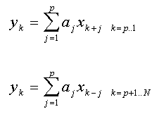
In these equations, x is the data series of length N and a is the autoregressive parameter array of order p. FlexPro uses the positive sign (linear prediction) convention for the AR coefficients. The model is defined as reverse prediction for the first p values, and forward prediction for the remaining N - p values. This definition is used for all AR fit statistics, although it is not the model fitted in any of the AR linear least-squares procedures. This model is only fitted if a non-linear AR-only fit is made in the ARMA procedure.
The ARMA definition is similarly one that preserves the degrees of freedom:
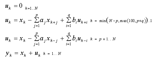
Here, b is the moving average parameter array of order q. The computations again start with reverse prediction, but a higher starting index is used to include a moving average in the first p values. This model is fitted in the non-linear ARMA algorithms.
AR Spectral Definitions
The AR and ARMA power spectral density functions are defined as follows:
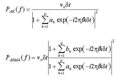
In these equations, ν is the driving white noise variance and δt is the sampling interval. Note that both spectral models are continuous functions of frequency.
Classes of AR Algorithms
The AR coefficients can be computed in a variety of ways. The coefficients can be computed from autocorrelation estimates, from partial autocorrelation (reflection) coefficients, and from least-squares matrix procedures. Further, an AR model using the autocorrelation method will depend on the truncation threshold (maximum lag) used to compute the correlations. The partial autocorrelation method will depend on the specific definition for the reflection coefficient. The least-squares methods will also yield results that are a function of how data are treated at the bounds (matrix size) as well as whether the data matrix or normal equations are fitted.
Most of the AR algorithms in FlexPro are least-squares procedures since these produce the best spectral estimates. Least-squares methods that offer in-situ separation of signal and noise through singular value decomposition (SVD) are the most robust of FlexPro’s AR methods. These algorithms are built into the AR procedures (there is, for example, no separate Principal Component AutoRegressive or PCAR option).
AR Prediction Models
A continuous function of time needs only the computed parameters of the model to produce an estimate for any value of time desired. Whether the original time sampling is uniform or irregular is not a factor once the model is generated. This is not true for an autoregressive model. An AR linear prediction model is a discrete function that requires uniformly sampled data.
When an AR model is evaluated in the time domain for a future predicted value, the last portion of the data sequence is filtered by the AR coefficients to generate a new element. Although an AR linear prediction model does not explicitly contain a noise component, this is intrinsically a part of the data sequence. White noise is thus managed, provided it is uncorrelated, point to point.
AR Model Limitations
In practice, it may not be possible to predict a present value from past values. The process may be stochastic (truly random) rather than deterministic. There may be no correlation between past values and the current one.
Nor is the background noise necessarily white and uncorrelated. Geophysical processes, for example, are often characterized by red noise backgrounds. For red noise, the variance decreases with increasing frequency. In some cases, the overall noise trend can be approximated by a first order AR model.
As an AR model order increases, more of the trends in the data series are incorporated. When noise is completely absent, pure harmonics are captured with an order equal to twice the number of components. More commonly, though, some level of noise is present.
Further, the narrowband signals are often anharmonic. The signal components will be close to harmonic, evidencing regular oscillations, but cannot be described by a single sinusoid or exponentially-damped sinusoid. The information necessary to describe the oscillatory trend may require that the AR model capture several cycles of the oscillation. For slowly changing patterns, this can mean appreciable model orders.
AR Signal-Noise Separation
A basic AR model fit does not offer effective signal-noise partitioning. Even if pure sinusoids are embedded in modest levels of noise, it may require an order well beyond twice the signal component count to successfully capture and spectrally render the sinusoids. In other words, if a model order is too low, only a portion of the deterministic signal is captured. The remainder is treated as part of the white noise. Spectral components are thus missed.
On the other hand, if a model order is too high, the full deterministic signal is captured but some measure of the noise is also modeled. Spurious spectral peaks can result.
There are three ways to manage this limitation. First, the noise can be filtered or removed prior to analysis. Second, an optimum AR order can be determined that captures all of the deterministic signal elements and includes as little noise as possible. The third option consists of an in-situ noise removal within the least-squares procedures that generate the coefficients. This last option is recommended.
Signal Eigenmode Selection
Rather than struggle to find an optimum model order, an explicit signal-noise separation can be made. As the AR order increases, there are more coefficients to map both data trends and noise. If a matrix procedure based upon principal components is then used, the initial eigenvectors will describe only the signal components. The latter eigenvectors will capture the noise contributions. Model order is then less important, since the noise vectors are discarded prior to the computation of the AR coefficients.
This in-situ signal-noise separation is accomplished using singular value decomposition (SVD) in the least-squares AR models. This option is found in all of the AR and ARMA procedures that utilize SVD. The retained eigenmodes should represent the signal or principal components since these are used for the procedure's solution. The discarded eigenmodes should represent the noise since this information is zeroed and does not factor into the solution. This signal-noise separation is intrinsic to SVD procedures. For narrowband component analysis, note that two signal eigenmodes are needed for each sinusoid. If a signal contains three principal harmonic components, the signal subspace should be set to six.
AR Continuous Spectra
Frequency domain AR spectra do not involve filtering of the original series except to determine an overall global measure of white noise. This is why AR frequency spectra are so smooth. The AR coefficients ideally model only the trends in the data while the noise is treated as a constant equal in value to the white noise variance or error power determined from the fitting. The AR frequency transform uses only the AR coefficients and this white noise variance, and the result is a continuous function of frequency.
Each FlexPro AR algorithm thus produces a white noise variance estimate. This variance impacts the magnitude, but not the shape of spectral components. Errors in estimating this white noise variance are translated to errors in scale of the AR spectral values. The Burg and Autocorrelation algorithms usually generate normally distributed prediction errors and AR spectra whose integral is very close to the power of the data. The least-squares procedures may not do so.
A successful AR fit to the signal components within the data can often be achieved using very short data records, and a very high resolution spectrum can result. An AR spectral estimator can consist of exceedingly sharp peaks, and for the better algorithms, these will be present at close to the exact frequency of the narrowband component. In an AR model, the frequencies are determined directly from the AR roots of the model. There is no need for a local maxima detection procedure.
In comparing AR and FFT methods, the latter are decidedly straightforward and robust. An FFT may need some optimization in terms of window selection, segment length and overlap, or zero-padding, but it is difficult to get an incorrect answer. Further, most of the refinements needed to fine-tune an FFT algorithm are intuitive. This is not necessarily true for AR spectra.
See Also
Spectral Estimators Analysis Object - AR Spectral Estimator
Spectral Estimators Analysis Object - ARMA Spectral Estimator