DCRemovalFilter (FPScript)
Removes the DC offset (DC bias) with the help of a digital (recursive) high-pass filter.
Syntax
DCRemovalFilter(DataSet, [ CutOffFrequency = 0.01 ], [ SamplingRate ], [ Order = 1 ] [ , PhaseCorrection = True ])
or
DCRemovalFilter(Result, [ CutOffFrequency = 0.01 ], [ SamplingRate ] [ , Order = 1 ])
The syntax of the DCRemovalFilter function consists of the following parts:
Part |
Description |
||||||||
|---|---|---|---|---|---|---|---|---|---|
DataSet |
The data set from which the DC offset is to be removed. Permitted data structures are data series, data matrix, signal und signal series. All numeric data types are permitted. If the argument is a list, then the function is executed for each element of the list and the result is also a list. |
||||||||
CutOffFrequency |
The cut-off frequency of the high-pass filter. The frequency must be between 0 and 0.25 (one fourth of the sampling rate normalized to one) or between 0 and 0.25 * SamplingRate. The cut-off frequency is defined as the frequency at which the filter amplitude exceeds 70.7 percent of the original signal amplitude. Permitted data structures are scalar value. All real data types are permitted, except calendar time und time span. The value must be greater or equal to 0. If the argument is a list, then the first element in the list is taken. If this is also a list, then the process is repeated. If this argument is omitted, it will be set to the default value 0.01. |
||||||||
SamplingRate |
Specifies the sampling rate. The argument is optional. If this argument is not specified, a normalized frequency from 0 to 0.25 must be specified as the cut-off frequency for CutOffFrequency. Permitted data structures are scalar value. All real data types are permitted, except calendar time und time span. The value must be greater than 0. If the argument is a list, then the function is executed for each element of the list and the result is also a list. |
||||||||
Order |
Specifies the order of the DC removal filter. Orders from 1 to 5 are allowed. Increasing the order causes an increase in the steepness of the high-pass filter. High orders, however, can cause numerical instabilities when using the filter with a cut-off frequency that is too low. Permitted data structures are scalar value. All integral data types are permitted. The value must be greater or equal to 1 and less or equal to 10. If the argument is a list, then the first element in the list is taken. If this is also a list, then the process is repeated. If this argument is omitted, it will be set to the default value 1. |
||||||||
PhaseCorrection |
The value TRUE specifies that filtering includes phase correction, which means the phase of the filtered signal is the same as that of the input signal. Filtering takes place twice in this case: once forward and once backward. Permitted data structures are scalar value. Supported data types are Boolean value. If the argument is a list, then the first element in the list is taken. If this is also a list, then the process is repeated. If this argument is omitted, it will be set to the default value True. |
||||||||
Result |
Specifies whether the filter coefficients or poles and zeros of the filter are returned as the result. The argument Result can have the following values:
If the argument is a list, then the first element in the list is taken. If this is also a list, then the process is repeated. |
Remarks
The filter corresponds to a Butterworth high-pass filter with the specified order Order and cut-off frequency CutOffFrequency. Alternatively, the Butterworth high-pass filter can also be created using the IIRFilter function.
Use the first syntax to remove the offset directly from signals. The structure of the result corresponds to that of the DataSet argument. In the case of data matrices and signal series, the calculation is made on a per column basis. If present, the X or Z components are copied to the result unchanged.
Use the second syntax to return the numerator and denominator coefficients of the filter as a list with two elements b and a, or the poles and zeros of the filter. The numerator and denominator coefficients can be used to calculate the filter amplitude response using AmplitudeResponse or the phase response using PhaseResponse .
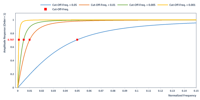
The filter has the following amplitude response (Order = 1) for different cut-off frequencies. The DC component is filtered out and the frequencies above the cut-off frequency are transmitted almost unattenuated::
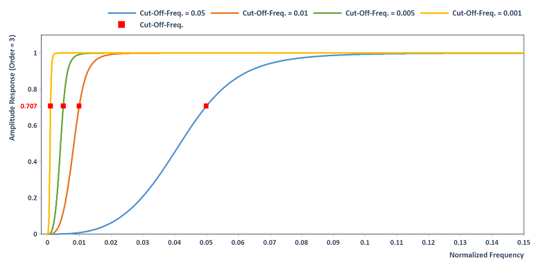
Increasing the order causes an increase in the steepness of the high-pass filter, for example when selecting Order = 3:
Note For the default setting Order = 1, the filter is reduced to a common recursive first order filter for removing the DC offset, also known as the Cascaded Differentiation Integration Filter; see [1, section 13.23] or [2]. Interpretation of this name: The Cascaded Differentiation Integration Filter is formed of backward differentiation, followed by subsequent "leaky" integration with feedback constant . The digital differentiator removes the DC component, and the subsequent integrator returns the input signal without the DC offset. The Cascaded Differentiation Integration Filter (CDI) has the following recursive definition rule:
![]()
The parameter from the interval [0, 1] can be calculated uniquely by the normalized cut-off frequency ω from the interval [0, 1/4] as follows:
![]()
Available in
FlexPro Basic, Professional, Developer Suite
Examples
DCRemovalFilter(DataSet)
Removes the DC bias of a data set. The normalized cut-off frequency is usually set to the normalized frequency of 0.01. This corresponds to a cut-off frequency of one hundredth of the sampling frequency.
DCRemovalFilter(DataSet, 3 Hz, SamplingRate(Signal.X))
Removes the DC bias of a data set. The cut-off frequency is set to 3 Hz. This is a normalized maximum frequency of 3 Hz / sampling frequency.
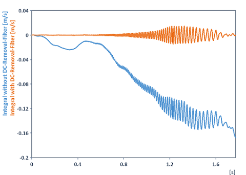
Integral(DCRemovalFilter(Signal))
Integrates a signal and removes the drift or offset (DC component) in advance. Reason: The reason for this signal drifting after integration is not only the accumulation of the offset during integration, but also the integrator’s inversely proportional amplitude response of the integrator (see Integral function). This amplifies the noise at frequencies close to the offset (DC component) and integration raises it to arbitrarily high values. The integrated curve then drifts away. To prevent this drifting, it is not enough just to subtract the mean, but frequencies close to the DC component also need to be cut off using a high-pass filter. The following illustration clarifies the situation (here of one of the acceleration signals from the FlexPro example files under C:\Users\Public\Documents\Weisang\FlexPro were integrated):
Dim coeff = DCRemovalFilter(FILTER_COEFFICIENTSCASCADED, 0.01, , 3)
AmplitudeResponse(coeff, 100000)
Calculates the amplitude response (with 100000 data points) of the DC removal filter for the normalized cut-off frequency of 0.01 and order of 3 with the help of the AmplitudeResponse function.
Dim coeff = DCRemovalFilter(FILTER_COEFFICIENTSCASCADED, 0.01)
Filter(Signal, coeff, TRUE)
First the numerator and denominator coefficients of the filter are calculated and then the data is filtered using the Filter function. The code is equivalent to: DCRemovalFilter(Signal).
Dim param = DCRemovalFilter(FILTER_POLESANDZEROS, 0.001, , 5)
Signal(Imag(param.Poles), Real(param.Poles))
Calculates the poles of the filters for the normalized cut-off frequency of 0.001 and order of 5 and returns them as signal. It should be noted that an order that is too high can cause numerical artifacts for cut-off frequencies that are too low. The numerical artifacts are mathematically conditioned by the fact that the poles of the filter are on the unit circle or come very close. For example, for Order = 1 the poles are farther from the unit circle than in the case of Order = 5. The most numerically stable filter is obtained for Order = 1.
See Also
Signal Analysis - Analysis Object
References
[1] Richard G. Lyons: Understanding Digital Signal Processing (3rd Edition). Prentice Hall,2011.ISBN 0-13-702741-9.
[2] Richard G. Lyons, Randy Yates: DC Blocker Algorithms. In: IEEE Signal Processing Magazine, Vol. 25, Issue 2. 2008.