Hilbert (FPScript)
Calculates the Hilbert transform. Frequently used for calculating instantaneous amplitude or instantaneous frequency as well as for the demodulation of signals.
Syntax
Hilbert(Signal [ , FFTLength = 0 ])
The syntax of the Hilbert function consists of the following parts:
Part |
Description |
|---|---|
Signal |
The real data set from which the analytic signal is to be calculated. The data set should be equidistantly sampled, since the algorithm uses the discrete Fourier transform (for equidistant data). Permitted data structures are data series, data matrix, signal, signal series und signal series with two-dimensional X-component. All numeric data types are permitted, except calendar time und time span. Void values are not permitted in this argument. If the argument is a list, then the function is executed for each element of the list and the result is also a list. |
FFTLength |
The length of the Fourier transform which is required for calculating the Hilbert transform. The FFT length must be longer than or equal to the data length. If the specified FFT length is longer than the data length, then zeros are appended for the internal Fourier transform. A value of -1 sets the FFT length to equal the next highest power of 2. The default value of 0 sets the FFT length to equal the data length. Permitted data structures are scalar value. All integral data types are permitted. The value must be greater or equal to -1. If the argument is a list, then the first element in the list is taken. If this is also a list, then the process is repeated. If this argument is omitted, it will be set to the default value 0. |
Remarks
The result has the same structure and unit as the argument Signal.
For aggregate data structures, only the Y component is considered. If present, the X or Z components are copied to the result unchanged. In the case of data matrices and signal series, the calculation is made on a per column basis.
The Hilbert transform is defined by a linear integral transformation for a (real or complex valued) signal x(t) as follows:
![]()
By this definition, in the equivalent form as a convolution, the Hilbert transform can likewise be written as:
![]()
By applying the Fourier transform to the last equation, the transfer function H of the Hilbert transform is calculated as follows:

In other words, the Hilbert transform can be interpreted as a phase shift by -π/2 (i.e. -90 degrees) for positive frequencies and by π/2 (i.e. 90 degrees) for negative frequencies. For instance, the Hilbert transform of the cosine function produces the sine function as the result.
For reference, refer to [1] as well as [4].
Application: Instantaneous amplitude, instantaneous phase, instantaneous frequency, envelope as well as demodulation of signals
The Hilbert transform is frequently used to calculate instantaneous quantities of the original signal: the instantaneous amplitude, instantaneous phase and instantaneous frequency. In addition, the instantaneous amplitude results in the upper envelope of the signal to be analyzed.
Using these instantaneous quantities, the signals can also be demodulated (amplitude modulation, phase modulation and frequency modulation).
The calculations, however, are based on the analytic signal derived from the Hilbert transform and not directly on the Hilbert transform.
Details, definitions and examples can be found in the Online Help covering the AnalyticSignal function or the Instantaneous Quantity Analysis Object.
Theoretical background: The algorithm for calculating the Hilbert transform.
The aforementioned continuous-time algorithm defines the transfer function H in the frequency range. The algorithm for calculating the discrete Hilbert transform is therefore (with the help of the FFT and discrete transfer function H) completed similarly to the algorithm of the AnalyticSignal function (also compare to [1]):
The only difference is in the definition of the transfer function.
The transfer function is now specified for even FFT lengths as: H[k] = 2 for k = 1, 2, ..., FFTLength/2 - 1 (positive frequencies) and H[k] = 0 for k = FFTLength/2 + 1, ..., FFTLength (negative frequencies). i in this case is the imaginary unit. Symmetrical coefficients k = 0 and k = FFTLength/2 are special. For these, H[k] = 0.
The transfer function is specified similarly for uneven FFT lengths as: H[k] = i for k = 1, 2, ..., (FFTLength-1)/2 and H[k] = i for k = (FFTLength-1)/2 + 1, ..., FFTLength as well as additionally H[0] = 0.
The FPScript algorithm for calculating the discrete Hilbert transform corresponds to the FPScript algorithm of the AnalyticSignal function with the exception of defining the transfer function. Similar code can be found in the Online Help covering the AnalyticSignal function.
Influence of FFT length: Using zero padding, i.e. by selecting the FFT length as greater than the data length, the resolution of the FFT required for the algorithm is increased. The calculation result can thus be improved. The following example clarifies this.
Note A real value signal x(t) can now be transformed into complex signal z(t) using the Hilbert transform as follows: ![]()
The transfer function of this transformation corresponds to the transformation from the definition of the AnalyticSignal function. The Hilbert transform can equivalently be defined as the imaginary part of the analytic signal associated with signal x(t).
Available in
Option Spectral Analysis
Examples
Imag(AnalyticSignal(realSig))
Results in the Hilbert transform of a real value signal. The code is equivalent to Hilbert(realSig).
realSig + 1i * Hilbert(realSig)
Transforms a real value signal into an analytic signal whose imaginary part results in the Hilbert transform. The code is equivalent to AnalyticSignal(realSig).
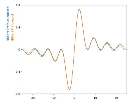
Dim t = Series(0, 10, 0.005)
Hilbert(Signal(Cos(t), t))
Calculates the Hilbert transform of the cosine function. The result is the sine function.
Dim t = Series(-25, 25, 0.005)
Dim sig = Signal(Sinc(t), t)
Dim hilbTrafo = Hilbert(sig, NumberOfRows(sig))
List("Hilbert Trafo calculated", hilbTrafo, "Hilbert Trafo exact", Signal((1-Cos(t))/t, t))
Calculates the Hilbert transform of the Sinc function. The exact result is included in the output, which is provided by the function 1/t - Cos(t)/t. The comparison is displayed in a 2D diagram:
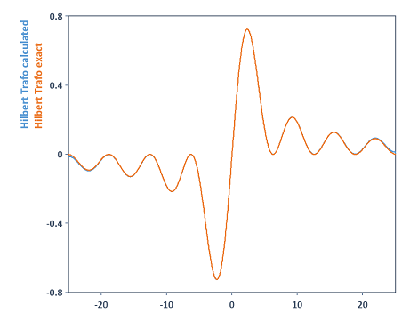
If you increase the FFT length in this example for the calculation of the variable hilbTrafo to 131072, for instance, the result in this case is a more precise calculation for the Hilbert transform. Both curves are now almost completely in agreement:
See Also
Instantaneous Quantity Analysis Object
References
[1] S. Lawrence Marple, Jr.: Computing the Discrete-Time "Analytic" Signal via FFT. In: IEEE Transactions on Signal Processing, Vol. 47, No.9. http://ieeexplore.ieee.org/iel5/78/16975/00782222.pdf?arnumber=782222,1999.
[2] B. Boashash: Estimating and Interpreting the Instantaneous Frequency of a Signal-Part I: Fundamentals. In: Proceedings of the IEEE, Vol. 80, No. 4, pp. 519–538. 1992.
[3] Bernard Picinbono: On Instantaneous Amplitude and Phase of Signals. In: IEEE Trans. Signal Processing, Vol. 45, No. 3. http://citeseerx.ist.psu.edu/viewdoc/summary?doi=10.1.1.178.833,1997.
[4] Oppenheim, Alan V., Ronald W. Schafer, and John R. Buck: Discrete-Time Signal Processing, 2nd Ed.. Upper Saddle River, NJ: Prentice Hall,1999.