Digital Filters Tutorial
This tutorial is concerned with FIR filter design and IIR filter design in FlexPro.
Signal Example
Using the Signal analysis object, we will generate a synthetic signal that will provide a very good demonstration of filter properties. Select Insert[Data] > Signal > Swept-Frequency Cosine. Setup the swept-frequency cosine function with the frequency of 1 and the second frequency of 10000. On the Sampling tab, determine the X component with a starting value of 0, a final value of 0.5 and a number of values of 1000.
IIR Filters
Highlight the Signal data set.
Click on Insert[Analyses] > Analysis Wizard.
Select the IIR Filters category under Filters. Next, select IIR Filter. Click on Next.
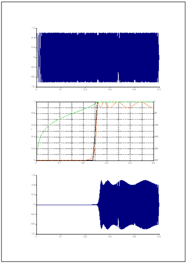
Step 2 of the Analysis Wizard contains an interactive dialog where you can select different filter types and filter characteristics. Three diagrams are presented in the Analysis Wizard preview window. You can see the input signal, the filter specification and the filtered signal or a diagram with the filter coefficients. You can use the option Show amplitude response to display or hide the amplitude response in the diagram using the filter specification. The amplitude response is also displayed in logarithmic representation.
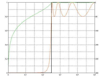
Select the highpass filter type and the Chebychev filter characteristics. This filter makes it possible to influence the ripple in the passband. Enable the option Use normalized frequencies. Select the Order 7 filter specification, the normalized cut-off frequency of Fc1 0.25 and the value 0.2 as the Passband Error. Now note that the generated filter specification shows that the filter's ripple moves in the passband in the range from 0.8 to 1, showing a maximum error of 0.2. If you reduce the ripple, this moves in the width of the transition at the expense of the filter steepness.
Unlike the Chebyshev filter, the ripple in the stopband is specified for the Inverse Chebyshev filter. The filter design for the Cauer filter is even more flexible, since both the ripple in the passband and the ripple in the stopband can be defined.
A fixed filter order can be specified for the IIR filters. In addition, it is also possible to calculate the filter order with regard to the defined specification. Instead of the normalized cut-off frequency, a lower and upper limit is specified for a transition. Moreover, both the passband error and the stopband error are specified. According to the specification, the filtered signal is not permitted to rise above or fall below these errors at the defined band limits.
Select Calculate as the order, and as the transition select the normalized frequencies 0.24 and 0.26. For each of the two errors, enter 0.1. Instead of the errors, you can also specify the ripple in the passband or the stopband attenuation in decibels. If you change the mode, the values will be converted accordingly.
Analysis Wizard Output Options
To view the objects that the FlexPro Analysis Wizard can automatically create, click on Next. In Step 3, check the two active options and then click Finish.
Seven objects are created in the FlexPro project database.
IIRFilter is the analysis object. This is the object that performs the filtering. Double clicking on this object opens the object.
Specification is the formula for creating the specification used for the representation.
Amplitude Response is the formula for creating the filter's amplitude response, which is also used for the representation.
The Signal diagram contains the input signal, the IIRFilter diagram is the representation of the filtered signal or the filter's coefficients, and the Specification diagram depicts the filter specification.
The IIRFilter document contains the three generated diagrams.
The IIR filter order is limited to 10, since higher orders can lead to instability. Therefore, let's now take a look at the FIR filter design, which permits higher orders and is also more flexible than the IIR filter design.
FIR Filters
Unlike the IIR filter design, there are two different calculation methods available for the FIR filter design: the filter design by windowing and the FIR Equiripple algorithm (Parks-McClellan method).
FIR Filter Design by Windowing
We will once again use the synthetic signal. Highlight the Signal data set.
Click on Insert[Analyses] > Analysis Wizard.
Select the FIR Filters category under Filters. Next, select Window Method. Click on Next. Select Filtered signal as the Result and Bandpass as the Filter type. Enable the option Use normalized frequencies. Use the Hamming window with the cut-off frequencies of Fc1 equal to 0.1 and Fc2 equal to 0.4 and a filter length of 71. Click on Finish. If you now highlight the input signal and the filter object you just created and create a line diagram, you will notice a phase shift between the two signals. On the second page of the wizard, you can remove this phase shift by selecting Filtered signal with phase correction as the result. For FIR filters, there is a constant phase shift, which is dependent only on the filter length and sampling rate of the signal. Phase correction is also possible when designing IIR filters. However, phase correction in this case occurs when the signal is filtered twice: once forward and once backward.
Now highlight the signal again and go back to the wizard to design a filter using windowing. The different window types exhibit different attenuation behavior. When the option Show amplitude response is enabled, with the exception of the Generalized Hamming window, the stopband attenuation is drawn as a horizontal line in the diagram with the specification. The attenuation is fixed for the Rectangular, Bartlett, Hamming, Hanning and Blackman windows (Window Method). For the Generalized Hamming window, the stopband attenuation can be influenced with the Alpha parameter, which can be in the range between 0 and 1. The two most flexible windows are the Kaiser and Chebyshev windows, since here the third parameter can be calculated from two of the three filter length, attenuation and transition parameters.
On the second page of the wizard, select Filter coefficients for the result. In the lower diagram, the impulse response is now displayed (corresponding to the filter coefficients) instead of the filtered signal. To create a bandpass, select the Kaiser window with the cut-off frequencies Fc1 equal to 0.1 and Fc2 equal to 0.4. Under Calculate, select Filter length. Specify a filter with an attenuation of 20 dB and a transition of 0.01. With this method, we will obtain a filter length of 94.
Now we want to design a filter with the filter characteristics just described using the FIR Equiripple method to be able to compare the two methods for designing FIR filters.
FIR Filter Design Using the Equiripple Method
Select the FIR Filters category under Filters. Next, select Equiripple Method. Click on Next.
Select Filter Coefficients as the Result, Bandpass as the filter template and calculate the filter length. Enable the option Use normalized frequencies. In the list containing bands there are three bands predefined for a bandpass. The upper and lower band limit, the associated gain factors and the approximation errors or weighting can be entered for each band. The transition between a stopband and a passband is formed from the difference between the upper band limit of one band and the lower band limit of the next band. You can edit the individual values by double-clicking on the entries in the list. However, for the predefined filter templates, certain entries, such as the gain factors, cannot be accessed. Now add the following values to the list:
Band |
Fc1 |
Fc2 |
Fc1 Attenuation |
Fc2 Attenuation |
Error |
|---|---|---|---|---|---|
1 |
0 |
0.095 |
0 |
0 |
0.1 |
2 |
0.105 |
0.395 |
1 |
1 |
0.1 |
3 |
0.405 |
0.5 |
0 |
0 |
0.1 |
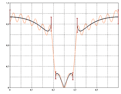
For this filter, a filter length of 77 is necessary when using the FIR Equiripple method. The passband and the stopband both have an equal ripple. The filters are therefore called equiripple filters. When designing IIR filters, an equal ripple in the passband and stopband is possible using the Cauer filter. However, the ripple in this case does not move in the range from 1±δ, but instead moves between 1-δ and 1.
With the FIR Equiripple method, optimal filters can be designed to meet the specification. Filters with a filter length lower than the filter design using windowing are the result. The other advantage of the FIR Equiripple method is that multiband filters can be designed as well.
Designing a Multiband Filter
For the multiband filter design, we will use a signal that contains four equal power reference sinusoids across the Nyquist range and three low power sinusoids placed between them. The low power components will be -40 dB, -50 dB, and -60 dB below the reference sinusoids. White noise will then be added so that a noise floor exists at approximately -75 dB.
The four reference sinusoids and three lower power sinusoids are defined as follows:
1.0*sin(2π*x*1005+π/2)+ (0dB)
1.0*sin(2π*x*2005+π/2)+ (0dB)
1.0*sin(2π*x*3005+π/2)+ (0dB)
1.0*sin(2π*x*4005+π/2)+ (0dB)
0.01*sin(2π*x*1505+π/2)+ (-40dB)
0.003162*sin(2π*x*2505+3π/2)+ (-50dB)
0.001*sin(2π*x*3505+π) (-60dB)
The x (time) values vary from 0 to 0.1 with a 0.0001 sample increment. The Nyquist frequency is thus 5000 (half the 10000 sampling frequency). The four reference sinusoids span the Nyquist range. The first low power sinusoid (-40 dB) has 1% of the amplitude and 0.01% of the power of one of the reference sinusoids. The next low power sinusoid (-50 dB) has 0.001% of the power of the references. The last of the test sinusoids (-60 dB) has only 0.1% of the amplitude and 0.0001% of the power of the reference sinusoids. Gaussian Noise at 0.15% was added to create a white noise floor at about -75 dB. This signal can also be found in the Spectral Analysis Tutorial.
Select the command File > Open Project Database and open the project database C:\Users\Public\Documents\Weisang\FlexPro\2021\Examples\Tutorials\Filter.fpd or C:>Users>Public>Public Documents>Weisang>FlexPro>2021>Examples>Tutorials>Filter.fpd. Select the Signal2data set. Click on Insert[Analyses] > Analysis Wizard. Select the FIR Filters category under Filters. Next, select Equiripple Method. Click on Next.
We will now design a multiband filter that filters out all signal components except the sinusoids at 1000 and 3000 Hz. To do this, select Filtered signal with phase correction as the result and Multiband as the filter template. Enable the option Use normalized frequencies. Calculate the filter length. Add as many bands to the list as necessary until there are a total of 5 bands available. Now add the following values to the list:
Band |
Fc1 |
Fc2 |
Fc1 Attenuation |
Fc2 Attenuation |
Error |
|---|---|---|---|---|---|
1 |
0 |
0.09 |
0 |
0 |
0.001 |
2 |
0.095 |
0.105 |
1 |
1 |
0.001 |
3 |
0.11 |
0.29 |
0 |
0 |
0.001 |
4 |
0.295 |
0.305 |
1 |
1 |
0.001 |
5 |
0.31 |
0.5 |
0 |
0 |
0.001 |
You can now save these entries as a filter template so that you can use them again at a later time. To do this, enter the name Multi1 under Filter Template and then press Save. If you later make another change to the list, you will have to re-save the entries. Click on Finish. FlexPro saves the templates in your user profile.
You can now check the result using a simple FFT. In addition, the Spectral Analysis Option gives you even more analysis options, such as creating a transfer function from the input signal and the filtered signal.
Designing Filters Using a Predefined Amplitude Response
At the end of the tutorial we will design a filter using the FIR Equiripple method, where the gain factors or amplitude response is specified as a data set. Highlight the data set Signal. Reopen the Analysis Wizard and select the FIR Filter Equiripple method. Next, set the following: custom filter template, calculate filter length, weighting from the list. Enable the option Use normalized frequencies. Define the following bands:
Band |
Fc1 |
Fc2 |
Error |
|---|---|---|---|
1 |
0 |
0.19 |
0.2 |
2 |
0.2 |
0.29 |
0.2 |
3 |
0.3 |
0.5 |
0.2 |
Now for the gain factor select the data set Amplitude. This data set contains an amplitude response, which was generated from an IIR bandstop (Cauer filter). If you now take a look at the specification, you will see that the filter specification is no longer defined by constants in the stopband and passband, but is instead defined by the specified data set.
It is also possible to define only a single band across the entire frequency range from 0 to 0.5. However, make sure that the individual bands do not have any points of discontinuity, since otherwise the algorithm cannot converge. In principle, we can say that designing the filter using a predefined amplitude response is very computation-intensive if the filter length is to be calculated. Moreover, depending on the predefined specification, the algorithm may not converge very well. In this case, the approximation errors are increased or the cut-off frequencies of the bands are changed.
The weightings of the bands can also be specified by a data set if the filter length is specified as fixed.
Filtering Multiple Input Signals
Using the Analysis Wizard, you also have the option of filtering multiple signals at the same time. To do this, select the signals to be filtered, open the Analysis Wizard and select Filtered Signal or Filtered signal with phase correction for the result. The Analysis Wizard generates an analysis object, which calculates the filter coefficients. In addition, for each input signal, an FPScript formula is created that filters the input signal using the calculated filter coefficients.
IIR/FIR Filter Comparison
In this tutorial, different design methods for IIR and FIR filters have been presented. This, of course, brings up the question as to which filters are preferred: IIR or FIR filters. Both filter types have advantages and disadvantages. It is therefore not possible to answer this question definitively. Below is a list of some points that may help you make a decision on which to use:
IIR Filters
Advantages:
•Simple calculation, since many frequency-selective filters with closed design formulas can be calculated.
•Specifying amplitude response is most efficient using IIR filters
•Less group delay compared to FIR filters
•Shorter filter length required
Disadvantages:
•No linear phase
•Variable group delay
•Only stable when all poles are within the unit circle
FIR Filters
Advantages:
•Option available for designing filters with a linear phase
•Always stable (contain only zeros in the transition function)
•Constant group delay
Disadvantages:
•Time-consuming iterative methods required
•Several coefficients are required to obtain steep filters (higher filter order required compared to IIR filters)
The FIR Equiripple method leads to lower order filters than the window method and offers more options for shaping (weighting, approximation errors) the filter specification. In addition, multiband filters can be designed using the FIR Equiripple method.
References
Excellent introductory references for digital filtering:
•Oppenheim, A. V. and Schafer, R. W. (1999). Discrete-Time Signal Processing, 2nd Edition. Prentice Hall, New Jersey.
•Antoniou, Andreas (2005). Digital Signal Processing. McGraw-Hill, New York.
The filter algorithms used in FlexPro are described in:
•J.H. McClellan, T.W. Parks, L.R. Rabiner. A Computer Program for Designing Optimum FIR Linear Phase Digital Filters. IEEE Transactions on Audio and Electroacoustics, Vol. AU-21, No.6, December 1973
•L. R. Rabiner, J. H. McClellan and T. W. Parks. FIR Digital Filter Design Techniques Using Chebyshev Approximation. Proceedings IEEE, Vol. 63, No. 4, pp. 595 610, April 1975
•L. R. Rabiner, C. A. McGonegal and D. Paul (1979). FIR Windowed Filter Design Program - WINDOW. Section 5.2 in Programs for Digital Signal Processing, IEEE Press, pp. 5.2-1 to 5.2-19.
See Also
FIR Filter Analysis Object (Window Method)