Spline (FPScript)
Interpolates a data set with a spline curve and samples this curve at definable points.
Syntax
Spline(DataSet, N, SamplingMode, [ V1 = 0 ] [ , Vn = 0 ])
or
Spline(Amplitude, Time, N, SamplingMode, [ V1 = 0 ] [ , Vn = 0 ])
The syntax of the Spline function consists of the following parts:
Part |
Description |
||||||||||||||||
|---|---|---|---|---|---|---|---|---|---|---|---|---|---|---|---|---|---|
DataSet |
The data set with a constant sampling interval, which is interpolated. If you specify a data series, then the X component will be generated automatically. Permitted data structures are data series, data matrix, signal, signal series und signal series with two-dimensional X-component. All numeric data types are permitted. For complex data types the absolute value is formed. If the argument is a list, then the function is executed for each element of the list and the result is also a list. |
||||||||||||||||
Amplitude |
The Y component of the signal to be interpolated. If you specify a signal, then its Y component is used. Permitted data structures are data series, data matrix und signal. All numeric data types are permitted. For complex data types the absolute value is formed. If the argument is a list, then the first element in the list is taken. If this is also a list, then the process is repeated. |
||||||||||||||||
Time |
The X component of the signal to be interpolated. If you specify a signal, then its Y component is used. Permitted data structures are data series, data matrix und signal. All numeric data types are permitted. For complex data types the absolute value is formed. If the argument is a list, then the first element in the list is taken. If this is also a list, then the process is repeated. |
||||||||||||||||
N |
Specifies the total number of points or per X interval of the signal. Permitted data structures are scalar value. All integral data types are permitted. The value must be greater or equal to 1. If the argument is a list, then the first element in the list is taken. If this is also a list, then the process is repeated. |
||||||||||||||||
SamplingMode |
Specifies how the calculated spline curve is to be sampled and which boundary conditions are used. The argument SamplingMode can have the following values:
...plus a constant, which determines the boundary conditions.
If the argument is a list, then the first element in the list is taken. If this is also a list, then the process is repeated. |
||||||||||||||||
V1 |
Determines the boundary condition at the start of the spline curve. Permitted data structures are scalar value. All real data types are permitted. If the argument is a list, then the first element in the list is taken. If this is also a list, then the process is repeated. If this argument is omitted, it will be set to the default value 0. |
||||||||||||||||
Vn |
Determines the boundary condition at the end of the spline curve. Permitted data structures are scalar value. All real data types are permitted. If the argument is a list, then the first element in the list is taken. If this is also a list, then the process is repeated. If this argument is omitted, it will be set to the default value 0. |
Remarks
The result always has the data type 64-bit floating point.
The result has the same unit as the argument DataSet.
A spline curve consists of cubic polynomials that are appended to one another to provide as smooth a course as possible.
The Y component of the data set to be interpolated must contain at least 3 values and the X component must be strictly increasing. If the latter is not the case (e.g., with a locus curve), then you should use theParametricSpline function. The X values, however, do not have to be equidistant. Before the spline interpolation, void values in the Y component are eliminated by linear interpolation.
You obtain a natural spline curve with V1 and Vn as second derivatives equal to zero.
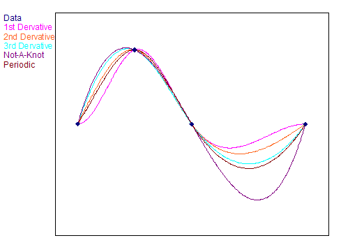
The following illustration shows spline curves with different boundary conditions. The values V1 and Vn are equal to zero respectively.
Available in
FlexPro Basic, Professional, Developer Suite
Examples
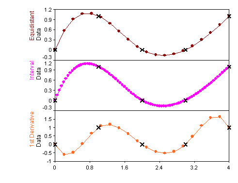
Spline({0, 1, 0, 0, 1}, 20, SPLINE_EQUIDISTANT)
Results in an equidistantly sampled spline curve with 20 values.
Spline({0, 1, 0, 0, 1}, 20, SPLINE_INTERVAL)
Results in a spline curve with 81 values.
Spline({0, 1, 0, 0, 1}, 20, SPLINE_EQUIDISTANT + SPLINE_1DERIVATIVE, -5, -5)
Results in an equidistantly sampled spline curve with 20 values. The curve has a gradient of -5 on the edges.
The following illustration shows the spline curves for the three examples:
See Also
Spline Interpolation Analysis Object
Surface Interpolation Analysis Object
References
[1] "Carl de Boor": "A Practical Guide to Splines, Revised Edition". "Springer-Verlag, New York",2001.ISBN 0-387-95366-3.