Fourier Spectral Analysis
Fourier Decomposition
The Fast Fourier Transform (FFT) decomposes a time-domain signal (which can be a function of time, spatial coordinates, or any time series abscissa) into complex exponentials (sines and cosines). A Fourier transform offers a complete picture of frequency space, but retains no information as to when in time a signal occurs. Thus a signal should either be wide-sense stationary, with a constant mean and variance across broad time segments, or you must care only qualitatively about whether a certain frequency content signal occurs somewhere in the time range being sampled.
The FFT is a fast algorithmic route for producing the Discrete Fourier Transform (DFT). The forward and reverse discrete transforms are defined as follows:
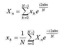
While the DFT is very simple, it is an order n² procedure. On the other hand, the FFT is an n*log2(n). The difference in processing times is dramatic with large data sets. FlexPro's best-exact-n FFT makes use of four different FFT algorithms.
Fourier decompositions are limited in resolution, as the frequencies at which the sines and cosines are computed are equally spaced and fixed in number. For a data set of n points, there will be n complex frequencies. For real data, the negative frequencies mirror the positive ones, and only the positive frequencies are displayed. Thus, n / 2+1 frequencies comprise the spectrum. Normalized frequencies range from 0, sometimes referred to as DC, to 0.5, the Nyquist frequency. The frequency 0 is the offset or mean value of the time signal and is often described as DC. The Nyquist frequency is the maximum frequency that can still be detected given the selected sampling rate. There are still two sampling values per period in the time signal for this frequency's signal components. FlexPro displays the actual frequencies. Normalized frequencies are used only if not time information is present in the data set.
Continuous Basis Functions
The Fourier decomposition represents a data sequence as a linear combination of a set of sine and cosinusoids. Although the data and Fourier sequences are each discrete, the basis functions are continuous and infinite in duration. It is thus possible to reconstruct the signal for any time within the range of the original sequence:
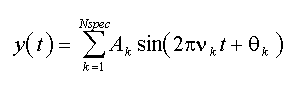
The Fourier basis functions can be treated as complex exponentials, zero phase sine and cosine pairs, phase bearing cosines, or phase bearing sines. In FlexPro, the Fourier basis functions are reported as phase bearing cosine elementary functions in a range from -π/2 to +π. In the above equation, A is the amplitude reported, ν is the frequency, and θ is the phase. The signal at any time t can be reconstructed by summing the value of all Nspec cosinusoids in the spectrum evaluated at that time. The amplitudes are adjusted so that all power is represented in the positive frequencies.
Spectral Leakage
Spectral leakage is the term used to describe the loss of power of a given frequency to other frequency bins in the FFT. Approximating a finite data stream with an infinite Fourier series assumes the data are fully periodic. Few data sets actually evidence this continuous wraparound property. Instead there are edge effects arising from the discontinuity at the bounds that cause spectral leakage. Spectral leakage also occurs as a consequence of the linear fixed frequencies used in the FFT.
Unless a sinusoid’s frequency just happens to correspond with the exact center of an FFT frequency bin, some portion of the signal will leak to other bins. One can expect, therefore, some portion of the adjacent bins to also reflect some measure of this peak. In fact, when a spectral component’s frequency is not centered in a bin, some portion of the variance due to this component may be accounted for by each bin in the spectrum. This tends to diminish as you get further away from the frequency of interest, although there will be harmonics. A sine and cosine at multiples of the original frequency, for example, would be expected to capture some of the variance as well.
From another viewpoint, an FFT can be considered a linear least-squares fit to sine and cosine functions at fixed linearly increasing frequencies. If a single sine wave is fit non-linearly, the parameters can be fully resolved since the amplitude, frequency, and phase can each vary in order to find the optimum. This is not possible in an FFT. While the amplitude and phase can vary, the frequencies cannot. Unless the frequency of the sine wave just happens to fall exactly at one of the FFT’s fixed frequencies, the sine component will be smeared across multiple frequencies.
While the spectral leakage attributable to the fixed frequencies is an intrinsic part of a Fourier spectrum, much can be done to eliminate edge effects. To produce the minimum spectral leakage, the data can approximate an infinite sequence by decaying to zero at both endpoints. This is accomplished by using a data tapering window.
Data Tapering Window
These windows are generally applied in the time domain, even when they are built within the frequency domain. This is because a simple multiplication is all that is needed to implement the tapering in the time domain. FlexPro offers a wide range of tapering windows with merit in signal processing.
A rectangular window (no actual window is applied) produces a one-sided bin width of 1.0 in the frequency domain. The data tapering windows in FlexPro vary in Fourier bin width from 1.1 to 6.0. Many popular windows have widths of 2.0, 3.0, and 4.0. When a data set is windowed, portions of the signal nearer the bounds are discarded, and resolution is degraded. A window with a bin width of 2.0 will have only one-half the resolution of its non-windowed counterpart. A window with a bin width of 4.0 will have only one-quarter the resolution.
Although some portion of the data’s influence is discarded or diminished, and despite the loss of resolution, windowed FFTs are often the best course for accurate estimation of spectral components, especially when a high dynamic range is needed. By having the data smoothly vary and decay to zero at the endpoints, spectral leakage is drastically reduced, so much so that a decibel (dB) scale, which is logarithmic, must be used to observe the spectral leakage across the bins in a meaningful way.
When an FFT processes data that have been tapered by a time domain window, each frequency bin effectively becomes wider. This width is sometimes referred to as the order of the window. The Hann and Hamming windows spread the signal across 2 bins and are thus order 2 windows. This spreading eliminates much of the spectral leakage associated with being too near an edge of a frequency bin. While there are a variety of window taper properties, the bin width is certainly the most important since this determines the resolution of the signal as well as the dynamic range the FFT is capable of representing. Each window has a characteristic shape which fixes most of the resolving properties of the resultant frequency spectrum. Some windows have an adjustable parameter, and for all of FlexPro’s data tapering windows, this controls the width of the peak in the frequency domain.
The control for most adjustable windows has been modified to directly reflect this bin width. Certain windows minimize the leakage at adjacent side lobes, at the cost of low to negligible frequency decay (rolloff) as you move further away from the peak in frequency. These windows give excellent resolution of closely spaced peaks of varying power in the spectrum, but may mask peaks of low power far from the peak frequencies. The Chebyshev window produces the narrowest possible peak for a specific side lobe (adjacent harmonic) leakage level. Other windows maximize the decay or rolloff of the spectral leakage, but are not as good at minimizing the leakage at nearby frequencies. Two peaks distant in frequency, each of low power, may be well detected, but in the case of two closely spaced peaks, one of greater power may fully mask one of lesser power.
There are thus two key design criteria in selecting a data tapering window. The first is resolution. Select the greatest bin width that offers acceptable resolution. The second involves selecting a window of that order based on whether or not you want to primarily resolve distant peaks of low power (where a maximum rolloff window is selected), or whether a low power peak may be in the shadow of a nearby component of greater power. Often a compromise is chosen. The best-known windows, such as the popular 4-parameter Blackman-Harris, Cos4 Blackman-Harris , tend to be those which minimize the adjacent side lobe spectral leakage.
The Flattop window represents a unique feature. This window has a main lobe maximum width of 5, thus offering a relatively low spectral resolution; however, the main lobe maximum has almost the same value within the complete band from one frequency line to its adjacent neighbor on the left and right. The main lobe maximum therefore shows a wide, but flat peak. This window is especially suitable for measuring powers or amplitudes of narrow-band signal components, i.e., individual peaks in a spectrum. Through the special type of main lobe maximum, the height of a peak is actually independent from its location between two frequency lines.
Periodogram Averaging
Data windows discard information near the bounds of the taper, emphasizing the spectral properties of data near the center of the record. If the data are truly wide sense stationary, the only problem is the additional variability arising from using only a portion of the data. The Periodogram is one spectral option that addresses this concern. In this procedure, a series of overlapped smaller segment windowed FFTs is averaged, reducing the variance at the cost of diminished spectral resolution.
Multitaper Analysis
Another algorithm that addresses the usage of information near the bounds of the data record is the Multitaper spectrum. In this procedure, the spectra from a set of orthogonal tapers are averaged. The spectrum resulting from a multitaper analysis is also of reduced variance, all of the data are represented, and spectral resolution is comparable to a full-size windowed FFT.
References
A good introduction to digital signal processing is:
•Oppenheim, A. V. and Schafer, R. W. (1989). Discrete-Time Signal Processing. Prentice Hall, Englewood Cliffs, NJ.
•H.D. Lüke (1985). Signalübertragung. Springer-Verlag Berlin, Heidelberg, New York. ISBN 3-540-15526-0.
The FFT Algorithms used in FlexPro are described in:
•C. Temperton, "Implementation of a Self-Sorting In-Place Prime Factor FFT Algorithm", Journal of Computational Physics, v. 58, p. 283, 1985
•R. C. Singleton, "An Algorithm for Computing the Mixed Radix Fast Fourier Transform", IEEE Trans. Audio Electroacoust., v. AU-17, p. 93, June 1969
•L. R. Rabiner, R. W. Schafer, C. M. Rader, "The Chirp z-Transform Algorithm and Its Application", BSTJ, 48, p.1249, May-June 1969
Information on data tapering windows is provided in:
•Albert H. Nuttall, "Some Windows with Very Good Sidelobe Behavior", IEEE Trans. ASSP, v29-1, Feb. 1981. 1981.
Information on multitaper spectra can be found in:
•Jonathan Lees and Jeffrey Park, "Multiple Taper Spectral Analysis", Computers and Geosciences, v21, p199, 1995.