Window Method
The design methods for FIR filters are based on direct approximation of the desired frequency response of the discrete-time system. For this method, the filter coefficients correspond to the impulse response of the filter to be designed. To be able to process different signals, it is necessary that these signals are finite. However, this is not always the case for all signals. The window method is often used to create these types of finite signal sequences from infinite sequences. This "cutting off" of an infinite sequence to create a finite sequence, however, affects the frequency range. This method would be precise in principle, but since only several finite values can be used, this principle leads to deviations which primarily limit the achievable slope steepness and stopband attenuation.
The approximation of an ideal filter by cutting off the ideal impulse response is identical to the convergence problem in Fourier series. Due to the behavior of Fourier series at points of discontinuity, a ripple always occurs in the passband and stopband. The ripple is inherently observed if a discontinuous function is modelled using Fourier series. The ripple also does not disappear when the number of coefficients is increased, but instead is concentrated only more strongly in the cut-off frequency range. This effect is known as the Gibbs phenomenon. A solution can be found through suitable weighting of the filter coefficients. The border coefficients are appropriately reduced. However, the filter order needed also increases for equal slope steepness.
Window Functions
The non-ideal effects, which are observed due to the finite number of filter coefficients, can be mitigated by using a weighting window. The principle of this is that the filter coefficients in the middle are more heavily weighted than the coefficients at the beginning and the end.
There are several window functions that define the maximum achievable stopband attenuation:
Windows |
Stopband attenuation [dB] |
Window attenuation (L in size) |
Window function w(i) |
|---|---|---|---|
Rectangular |
21 |
1 |
|
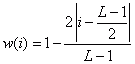
Bartlett (triangle) |
25 |
0.5 |
|
Hamming |
53 |
0.54 |
|
Generalized Hamming |
- |
Alpha |
|
Hanning |
44 |
0.5 |
|
Blackman |
74 |
0.423 |
|
Kaiser (γ = 2.12) |
30 |
0.78 |
|
Kaiser (γ = 4.54) |
50 |
0.569 |
ditto |
Kaiser (γ = 7.76) |
70 |
0.442 |
ditto |
Kaiser (γ = 8.96) |
90 |
0.412 |
ditto |
With this step, primarily the attenuation behavior is improved In return, however, the slope steepness is degraded and the signal undergoes an additional attenuation. For approximation, you can say that the more strongly the achieved stopband attenuation increases, the more the slope steepness is degraded at the same filter length L. Of course, the filter length can be increased again in order to improve the slope steepness.
The Kaiser windows are always the best choice with regard to achieved slope steepness/filter length and achieved stopband attenuation. In addition, there is a heuristic formula for the Kaiser filter, which estimates the necessary filter order from the stopband requirements.
A description of the Chebyshev window function (Dolph-Chebyshev Window) can be found in Antoniou, p.440.
Filter Design Method Using the Kaiser Window
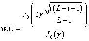
The Kaiser window fulfills a special purpose. The compromise between the width of the main lobe and the attenuation of the side lobe can be quantified by searching for a window maximally concentrated in the frequency range by ω = 0. Kaiser (1966, 1974) figured out that a virtually optimal window can be found using a modified Bessel function of the first type and zero order.
This window can be adjusted in such a way that a compromise can be found between the amplitude of the side lobe and the width of the main lobe. As with the Chebyshev function, the filter length L can also be calculated for the Kaiser window from the attenuation and transition data. The filter length is the smallest odd number that fulfills the following empirically determined inequation.
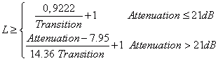
For instance, at least a filter length of 17 is necessary for a filter design with an attenuation of 30 dB in the stopband and a transition of 0.1 (normalized frequency).
Algorithm
The algorithm used in FlexPro is based on the FIR1 program by L.R. Rabiner, C.A. McGonegal and D. Paul.
References
•Oppenheim, A. V. and Schafer, R. W. (1999). Discrete-Time Signal Processing, 2nd Edition. Prentice Hall, New Jersey.
•Antoniou, Andreas (2005). Digital Signal Processing. McGraw-Hill, New York.
•L. R. Rabiner, C. A. McGonegal and D. Paul (1979). FIR Windowed Filter Design Program - WINDOW. Section 5.2 in Programs for Digital Signal Processing, IEEE Press, pp. 5.2-1 to 5.2-19.