Calculation of the Analytic Signal
Defining instantaneous amplitude, instantaneous phase and instantaneous frequency
By transforming the real input signal into an analytic signal, it is possible to derive and examine the local quantities of the original signal, the instantaneous amplitude, instantaneous phase and instantaneous frequency:
For this purpose, write the analytic signal z(t) in a polar graph as follows:
![]()
The instantaneous amplitude or instantaneous envelope is now defined as the amplitude a(t) of the analytic signal; i.e.:
![]()
If the original signal does not have a trend or offset, then it actually results in the amplitude response or the upper envelope of the signal to be analyzed.
The instantaneous phase is the phase of the signal Φ(t). The phase Φ(t) can be modeled in the following format:

The instantaneous frequency ω(t) is then therefore defined as::
![]()
For single-component signals without a trend or offset, these definitions actually result in the phase response as well as the frequency response of the signal to be analyzed.
For signals that have a trend or offset, all interpretations mentioned above are only correct when a signal trend correction is made. The following example clarifies these relationships:
Also refer to [2] and [3] for more information.
Applications: Calculating instantaneous amplitude, instantaneous phase, instantaneous frequency and envelope
Note: The following list of FPScript formulas used to calculate the instantaneous amplitude, instantaneous phase, instantaneous frequency form the basis of the Instantaneous Quantity Analysis Object. The following example can thus be evaluated in a similar manner with the Instantaneous Quantity Analysis Object.
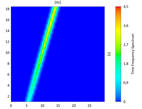
For the example, you first generate a swept frequency cosine with 10,000 values whose X component has the unit s, starting at 0 s and ending at 20 s. The starting frequency is 5 Hz and the ending frequency is 15 Hz. The amplitude of the swept frequency cosine is 1, the offset and start phase are each 0. Now scale the generated synthetic signal with the help of the following formula (called Data):
Dim amplitude = Sqrt(Value Signal.X + 1)
amplitude * Signal
The time-frequency spectrum of the scaled signal returns (visualized in a 3D contour diagram):
The signal does not have a trend. The format for the instantaneous amplitude calculation is therefore as follows:
Absolute(AnalyticSignal(Data))
As mentioned above, this now corresponds to the upper envelope (or the amplitude response) of the scaled signal:

The lower envelope is similarly obtained using:
-Absolute(AnalyticSignal(Data))
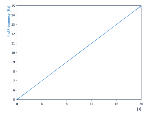
To calculate the instantaneous frequency, use the following FPScript code:
Dim instPhase = PhaseUnwrap(Phase(AnalyticSignal(Data)))
ChangeUnit(1/(2*PI)*Derivative(instPhase), "Hz")
This results in the frequency response of the signal:
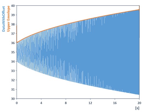
Now create a second formula (called DataWithOffset) in which an offset or trend is added: Example:
Data + 35
Note Note that to determine the amplitude response, phase response, frequency response or envelope (with the help of the algorithms above), correction of the trend or offset of the signal to analyze is necessary.
First recalculate the instantaneous amplitude. For instance, the trend correction can be done using the FPScript function Trend- or by way of floating mean values using the Mean-function:
Dim offset = Trend(DataWithOffset, TREND_CONSTANT)
Absolute(AnalyticSignal(DataWithOffset - offset))
This now actually results in the amplitude response of the signal scaled with an offset. However, to determine the envelope, the trend must then be added back in. The formula only needs to be slightly modified as follows:
Dim offset = Trend(DataWithOffset, TREND_CONSTANT)
Absolute(AnalyticSignal(DataWithOffset - offset)) + offset
This actually returns the upper envelope of the signal scaled with an offset:
Note that to determine the frequency response it is necessary to subtract the offset as well:
Dim offset = Trend(DataWithOffset, TREND_CONSTANT)
Dim instPhase = PhaseUnwrap(Phase(AnalyticSignal(DataWithOffset - offset)))
ChangeUnit(1/(2*PI)*Derivative(instPhase), "Hz")
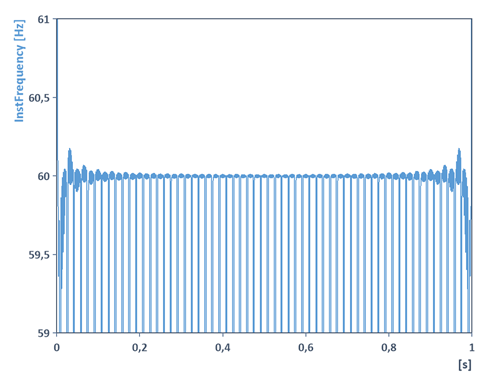
Note 1: When calculating the instantaneous amplitude, instantaneous phase, instantaneous frequency or envelope, on the edges of the signal (or generally in the vicinity of the jump discontinuities of the signal), side effects in the form of overshoots can occur. These overshoots cannot be avoided in the aforementioned algorithm and are purely mathematically determined. The cause is the Gibbs phenomenon, which causes overshoots in the vicinity of the jump discontinuities in the case of Fourier series and of the Fourier transform.
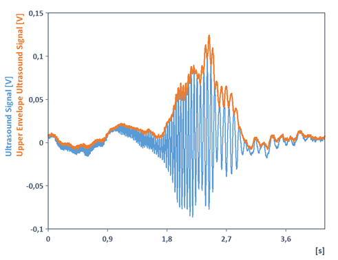
Note 2: For the following signal provided with the sample data from FlexPro, the aforementioned algorithm for determining the upper envelopes (with trend correction using the Mean function) results in the upper envelope. It is not required for the signal to be a single-component signal:
Note 3: It is important to note that in the case of multicomponent signals, the interpretations as instantaneous phase and instantaneous frequency no longer apply. Note the following FPScript code for this:
Dim x = Series(0 s, 1 s, 0.001)
Dim y = Sin(2 * PI * x * 30 Hz) + Sin(2 * PI * x * 90 Hz)
Signal(y,x)
In this case, the algorithm for determining the instantaneous frequency results in an averaging of the two sine frequencies:
Additional application: Demodulation of signals (amplitude demodulation, phase demodulation, frequency demodulation)
The thus defined instantaneous quantities can therefore also be used for demodulation of signals. For example, a modulated signal is provided as:
![]()
The instantaneous amplitude then actually results in the amplitude response a(t), whereas the instantaneous phase is calculated as Φ(t). In addition, the frequency response of the specified signal can be determined with the help of the instantaneous frequency.
Theoretical background: The algorithm for calculating the analytic signal.
The aforementioned continuous-time algorithm defines the transfer function H in the frequency domain. The algorithm for calculating the discrete analytic signal is therefore (with the help of the FFT and discrete transfer function H) implemented as described below; refer to [1] in particular:
The transfer function is specified for even FFT lengths as: H[k] = 2 for k = 1, 2, ..., FFTLength/2 - 1 (positive frequencies) and H[k] = 0 for k = FFTLength/2 + 1, ..., FFTLength (negative frequencies). Symmetrical coefficients k = 0 ad k = FFTLength/2 are special. For these, H[k] = 1.
The transfer function is specified similarly for uneven FFT lengths as: H[k] = 2 for k = 1, 2, ..., (FFTLength-1)/2 and H[k] = 0 for k = (FFTLength-1)/2 + 1, ..., FFTLength as well as additionally H[0] = 1.
The FPScript algorithm for calculating the analytic signal is therefore defined as follows (the argument FFTLength must be greater than or equal to the data length):
Arguments sig, FFTLength
Dim N = NumberOfRows(sig)
Dim fftInput = ComplexFloatingPoint64(sig.Y : (0 # (FFTLength - N)))
Dim fourierTrafo = FFTn(fftInput)
Dim H = 0 # FFTLength
H[0] = 1
If FFTLength Mod 2 == 0 Then
H[FFTLength/2] = 1
H[1, FFTLength/2 - 1] = 2
Else
H[1, (FFTLength - 1)/2] = 2
End
return Signal(IFFTn(H * fourierTrafo)[0, N-1], sig.X)
Influence of FFT length: Using zero padding, i.e. by selecting a FFT length greater than the data length, the resolution of the FFT required for the algorithm is increased. The calculation result can thus be improved. An example of this can be found in the Online Help covering the Hilbert-function.
References
[1] S. Lawrence Marple, Jr., "Computing the Discrete-Time "Analytic" Signal via FFT", IEEE Transactions on Signal Processing, Vol. 47, No.9. http://ieeexplore.ieee.org/iel5/78/16975/00782222.pdf?arnumber=782222,1999.
[2] B. Boashash, "Estimating and Interpreting the Instantaneous Frequency of a Signal-Part I: Fundamentals", Proceedings of the IEEE, Vol. 80, No. 4, pp. 519–538. 1992.
[3] Bernard Picinbono, "On Instantaneous Amplitude and Phase of Signals", IEEE Trans. Signal Processing, Vol. 45, No. 3. http://citeseerx.ist.psu.edu/viewdoc/summary?doi=10.1.1.178.833,1997.
See Also
Instantaneous Quantity Analysis Object