This analysis object allows you to approximate a circle, i.e. carry out circular curve fitting on the underlying data. Use circle approximation to analyze roundness measurements and to calculate shaft vibrations (see [1], [2] [4]). The LSCI, MCCI, MICI, MZCI circle approximation methods are available as well as an elementary circle approximation method (similar to ISO 7919-1 from [3]).

In addition, you can remove circular outliers from the data and use a Gaussian filter for smoothing prior to carrying out the circle approximation. The underlying data is also referred to below as the profile.

Description and Output Results

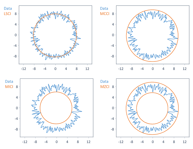
The LSCI, MCCI, MICI, MZCI circle approximation methods calculate one or more reference circles, which are determined differently depending on the method chosen:

Note  Depending on the circle approximation method selected, the center coordinates of the reference circles differ to a greater or lesser extent from each other.

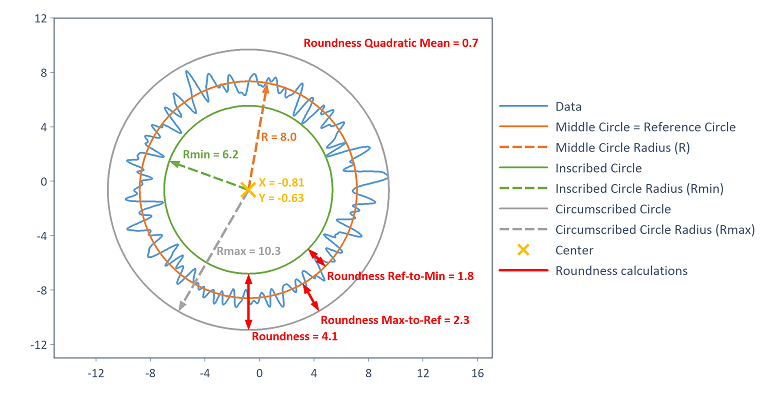
The center circle, inscribed circleand circumscribed circle are derived from the reference circle (or circles) and calculated (each with the same circle center as the reference circle). The analysis object can return the circles, statistical parameters (e.g. circle radii and circle center coordinates) and the prefiltered data as results. You can specify the number of values of circles as parameters.

In all cases the roundness is available as a statistical parameter (also called roundness deviation ). This is always calculated as the difference between the circumscribed circle radius and the inscribed circle radius (and is therefore a derived quantity from the respective reference circle). The roundness deviation is a measurement of the roundness of the measured profile. For the LSCI method and the elementary circle approximation method (determination of the circle center by averaging the circular path), additional statistical parameters are calculated and output as described below.

The following figure visualizes the output circles and statistical parameters for the example of the LSCI circle approximation method:

LSCI - Least Squares Circle

Calculating the LSCI reference circle is based on the LeastSquaresCircle function. The LSCI circle is calculated as the circle at which the sum of squares of deviations from the data becomes minimal. In the referenced literature this is referred to as a Gauss circle. The inscribed circle is then provided as the maximum inscribed circle related to the LSCI circle center. The reference circle is provided as the minimum circumscribed circle related to the LSCI circle center. The circumscribed circle corresponds to the reference circle, i.e. the LSCI circle.

The following two algorithms are available for calculating the LSCI circle:

In the LSCI method, in addition to roundness deviation, the peak-to-reference roundness deviation (difference between circumscribed circle radius and reference circle radius), the reference-to-valley roundness deviation (difference between reference circle radius and inscribed circle radius) as well as the root mean square of the deviations of the data points to the reference circle are output as statistical parameters (refer to [1]).

MCCI -  Minimum Circumscribed Circle

Calculating the MCCI reference circle is based on the MinimumCircumscribedCircle function. In this method, the reference circle is calculated as the circle with the smallest possible diameter that can be placed on the profile from the outside. This is also called a minimum circumscribed circle. The circumscribed circle in this method corresponds to the reference circle. The inscribed circle is provided as the maximum inscribed circle related to the reference circle center. The center circle in this case is also defined as the arithmetically averaged circle between the reference circle (i.e. circumscribed circle) and the inscribed circle.

To calculate the MCCI circle, the underlying algorithm requires calculation of the convex hull. The convex hull can be calculated using one of the following two methods:

MICI - Maximum Inscribed Circle

Calculating the MICI reference circle is based on the MaximumInscribedCircle function. In this method, the reference circle is calculated as the circle with the largest possible diameter that can be placed on the profile from the inside. This is also called a maximum inscribed circle. The inscribed circle in this method corresponds to the reference circle itself. The circumscribed circle appears as the minimum circumscribed circle related to the reference circle center. The center circle in this case is defined as the arithmetically averaged circle between the circumscribed circle and the reference circle (i.e. inscribed circle).

MZCI - Minimum Zone Circles

Two reference circles are determined in the MZCI method. Calculation is based on the MinimumZoneCircle function. In this case two concentric circles are determined which enclose the roundness profile and have the smallest possible radial distance from each other. The reference circles consist of the circumscribed circle and inscribed circle. The center circle in this case is defined as the arithmetically averaged circle between the two reference circles, i.e. the circumscribed circle and the inscribed circle.

To calculate the MZCI circle, the additional Iterations are derived from the Increment parameters are used. It is helpful to understand the MZCI algorithm in order to declare the parameters: The minimum zone concentric reference circles are estimated during the first iteration step by the inscribed and circumscribed circles calculated by the least squares circle (LSCI). The result is then improved iteratively. A new point is selected around the center point of the current concentric inscribed and circumscribed circles with the help of a two-dimensional normal distribution (standard deviation corresponds to the Increment). A check determines whether the concentric inscribed and circumscribed circles recalculated on the new point have less of a radius difference than before. If they do, the point becomes the new center point. The procedure is now repeated iteratively n times as per the value of the Iterations parameter and the minimum zone circles are thus improved successively.

The following options are available for the Iterations and Increment parameters:

determination of the circle center by averaging the circular path

This circle approximation method is very simple and involves determining the center of the circle by averaging the X and Y components. The center of the circle is therefore determined a priori. A reference circle is thus not determined using this method. The reference circle appears as the minimum circumscribed circle related to the calculated center of the circle. The inscribed circle appears as the maximum inscribed circle related to the calculated center of the circle. The radius of the center circle corresponds to the mean value of the distances of the data points from the center of the circle. This defines the center circle. It should be noted that the center circle calculated this way can be interpreted as the (initial) estimated value of the LSCI circle (and produces similar results). Using this method then only makes sense when the underlying data is periodically sampled (closed profile).

If reference circle(s) was selected as the result, all circles will be output (i.e. inscribed, center and circumscribed circle) instead, since there is no explicit reference circle for this method.

Note   This elementary circle approximation method follows the procedure from ISO 7919-1, where the center of the circle is also calculated by averaging the X and Y components (see [3]). However, please note that no inscribed, center and circumscribed circles are defined in ISO-7919-1 and consequently the roundness deviation, as specified above, was not calculated. Like the methods mentioned above, the inscribed, center and circumscribed circles as well as the roundness deviation are provided here as results for reasons of symmetry and comparison.

In addition, other statistical quantities are output which are listed in ISO 7919-1 as a measurement for calculating the shaft path. These are:

Prefiltering by removing circular outliers

Prior to carrying out the circle approximation, circular outliers can be removed from the data. All data points are removed whose distance from the specified circle center is greater than the adjustable minimum radius and shorter than the adjustable maximum radius :

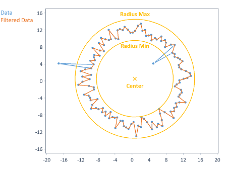
The X and Y coordinates of the circle center can either be calculated automatically (as the average of the respective X and Y component of the input data) or specified explicitly.

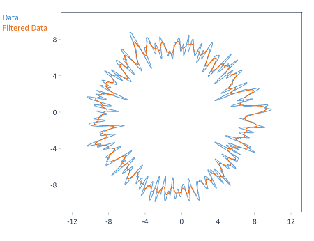
Prefiltering with a Gaussian filter

Prior to carrying out the circle approximation, the roundness profile can be prefiltered using a Gaussian filter (see [2]). The GaussianFilter function is used for this purpose. For mathematical reasons, the underlying data must be sampled periodically for filtering (i.e. closed profile).

The Gaussian filter is typically used in this case to smooth the profile (filter type setting: Low pass). Like [2], the Gaussian filter can likewise be used for high-pass filtering of the profile. A Gaussian band pass filter can be implemented by executing a low-pass and high-pass filter consecutively.

Specify the cut-off frequency for filtering in the unit UPR (Undulations Per Revolution). For example, 150 UPR is the 150th harmonic vibration of the fundamental frequency. The (normalized) fundamental frequency must also be specified. This is the reciprocal of the number of data points per revolution. The following options are available for specifying the Number of data points per revolution:

The following illustration shows a profile smoothed with a Gaussian filter (i.e. low-pass filtering) with a cut-off frequency of 50 UPR:

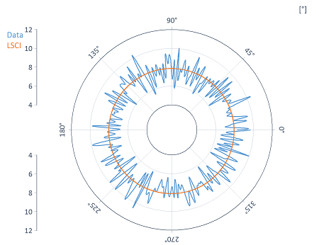
Data as polar coordinates

The input data may be present both in cartesian coordinates and polar coordinates (radius and angle). You can enter this on the Data tab of the analysis object. The Y component here is the radius and the X component is the angle.

The following settings are available for the Angle unit :

If a polar coordinate representation is present, the data are transformed into cartesian coordinates before the calculation.

The results, on the other hand, are always output in cartesian coordinates. You can transform them into a polar diagram for presentation as shown in the following example:

References

[1] DIN Deutsches Institut für Normung e.V.Part 1: Vocabulary and parameters of roundness (DIN EN ISO 12181-1:2011),Geometrical product specifications (GPS)- Roundness, 2011.

[2] DIN Deutsches Institut für Normung e.V.Part 2: Specification operators (DIN EN ISO 12181-2:2011),Geometrical product specifications (GPS)- Roundness, 2011.

[3] DIN Deutsches Institut für Normung e.V. Measurements on rotating shafts and evaluation criteria, Part 1: General guidelines (DIN ISO 7919-1:1996), 1996.

[4] Verein Deutscher Ingenieure. Form measurement - Principles for the measurement of geometrical deviations (VDI/VDE 2631), 1999.]

FPScript Functions Used

LeastSquaresCircle

MaximumInscribedCircle

MinimumCircumscribedCircle

MinimumZoneCircle

GaussianFilter

Frequency

ValuesInInterval

See Also

ConvexHull

* This analysis object is not available in FlexPro View and FlexPro Basic.