2D Approximation Analysis Object *
With this analysis object you can approximate an arbitrary model function Y(Y, Z) to your measurement data based on the least square error method.
You should use the approximation procedure if you know the mathematical relationship between your measurement data.
The result of the 2D approximation is a formula that describes the functional Y(X, Z) relationship between the Y, X and Z components of your data.
The quality of the calculated formula mainly depends on the model function, which you must specify as the basis for the 2D approximation. The model function is a linear combination of different element functions with the independent variables X and Z. FlexPro offers you over 25 of these element functions from which you can construct your linear combination. Alternatively, you have the option of defining your own element functions.
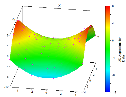
For the example above, for instance, the following model function is recommended: Y(X, Z) = p0 + p1 * X² + p2 * Z². For this you have to select the element functions Constant, X^2 and Z^2 on the Options tab of Standard Model Function. The coefficients p0, p1 and p2 of the linear combination are calculated so that the resulting formula approximates as closely as possible the specified source data.
FlexPro provides you with the quality of the approximation through a goodness-of-fit measure. It specifies how precisely the calculated formula approximates the source data, and this should be as small as possible. The goodness-of-fit measure, also known as χ² (Chi-squared), is equal to the sum of the squares of all deviations of the approximated model function of the data.
Standard and Custom Model Function
On the Standard Model Function tab, FlexPro offers you several predefined element functions. Simply select the functions that you want to use in the linear combination. The resulting model function will appear at the lower edge of the field.
If you want to use your own element functions, switch to the Custom Model Functions tab. Click on Add item and then choose either one of the predefined model functions or enter the element function you want to use. Write the function in FPScript notation, using the variables X and Z.
Dynamic and Static Approximation
The approximation offers you two alternatives for calculating the coefficients: You can calculate the factors once and enter them as static in the model function or choose a dynamic calculation for the factors. In this case, the factors are always re-calculated when the source data is changed.
Approximation and Approximation Coefficients
You can choose whether you want the approximation or the approximation coefficients as the result. The coefficients are output as a data series with the goodness-of-fit measure χ² as the last value in the series. The approximation, i.e. the sampled model function can be output as a space curve or signal series.
Evaluating the Approximated Model Function
You can evaluate the approximated model function at the same X and Z positions where your data points are located. Alternatively, you can freely define the X and Z values for which the function is to be evaluated. For this, on the Data tab you can enable the option Use a different data set as independent variable X or Use a different data set as independent variable Z and specify a data set for the X or Z values.
FPScript Functions Used
See Also
Surface Interpolation Analysis Object
* This analysis object is not available in FlexPro View.