Revolution Synchronous Order Tracking Analysis Object (Order Tracking Option)
The Rotation Synchronous Order Tracking analysis object calculates an order analysis for speed-dependent vibrations. Vibrations measured on rotating machines show a spectrum in which maxima occur at frequencies corresponding to a multiple of the machine's speed. There are two different causes for the occurrence of these maxima. On the one hand, the machine can be considered as a non-linear transmission system, which is excited with a harmonic vibration corresponding to the rotational speed. The non-linearity generates harmonics of this basic vibration, which lead to corresponding maxima. On the other hand, such a machine may contain components whose speed is not equal to the basic speed, but always corresponds to a fixed multiple of this speed. For example, different shafts in a gearbox have different speeds. But also the teeth of a gear or the balls in a ball bearing generate vibrations that are in a fixed relation to the speed. If this ratio of the fundamental frequency of a component to the fundamental frequency of the machine is known as the order, then individual maxima in the spectrum can be specifically assigned to a single or a few components of the machine. This can be used, for example, to isolate the cause of resonances.
In the method used here, a sampling rate conversion of the time signal is first performed (revolution synchronous resampling) so that the signal is no longer present in temporally equidistant steps, but in equidistant rotation angle steps (i.e. equidistant rotation intervals). This provides an effective method for performing order tracking, since the frequency spectrum (i.e. the Fourier Transform) of the signal converted to the revolution domain then provides the so-called order spectrum directly (for details, refer to RevolutionSyncSampling):
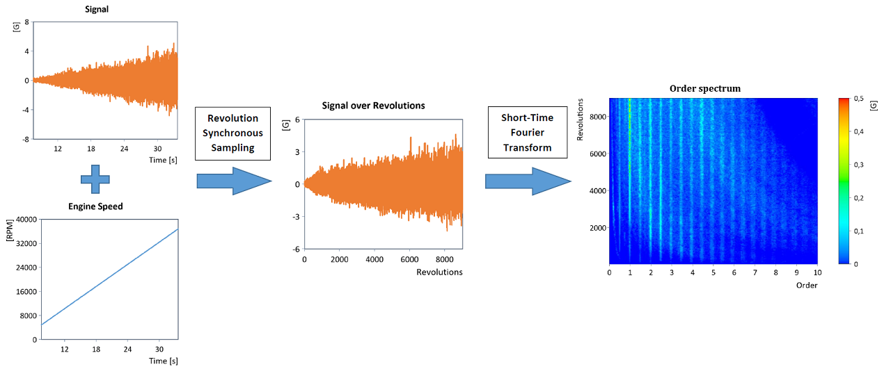
The order curves are then obtained from the order spectrum by extracting the individual order lines (order cuts).
Two measurement methods are predominantly used for order tracking. During a ramp-up, the vibration and the instantaneous speed are measured synchronously, while the machine is usually ramped up slowly from its minimum to its maximum speed (run-up analysis). In a second method, the machine is first brought up to a certain speed and then a vibration measurement is taken for this speed (order tracking with constant speed). The Revolution Synchronous Order Tracking analysis object supports both variants. In addition, order analysis using revolution-synchronous resampling is extremely flexible and can even be performed for noisy as well as non-monotonic speed data sets (order tracking with variable speed).
Data tab
This tab specifies the input data and parameters for transformation from the time to revolution domain (for details, also see RevolutionSyncSampling):.
Signals in the time domain
The time signal to be analyzed for the analysis object must be in the data structure Signal. The Speed can either be stored in the Signal data structure (corresponds to a run-up analysis with variable speed) or as a scalar value (corresponds to order tracking with constant speed or to a fixed fundamental frequency).
If there are no units or unit management is switched off, the speed is always interpreted in the unit [1/min] (rpm) and the X component of the time signal is interpreted in the unit .
The instantaneous speed is often measured with a pulse encoder, which records a certain number of pulses per revolution. You can convert the resulting pulse signal directly into a speed signal. To do this, select the option Speed is pulse signal and enter the Number of pulses per revolution. The conversion of the pulse signal into a speed signal is done with the ImpulseToFrequency function.
Resampling into the revolution domain
Three different modes are available for resampling from the time to the revolution domain. In most practical applications, the linear resampling is sufficient:
Resample method |
Description |
|---|---|
Linear interpolation |
The time signal is evaluated at the (non-equidistant) time points of the equidistant revolution sampling points by means of linear interpolation before being transformed into the revolution domain. This makes the transformation fast, but can cause aliasing in the subsequent calculation of the order spectrum. |
Spline interpolation |
The time signal is evaluated at the (non-equidistant) time points of the equidistant revolution sampling points by means of spline interpolation before being transformed into the revolution domain. Compared to linear resampling, spline interpolation is slightly slower, but aliasing is reduced. |
FFT resampling |
The time signal is evaluated by FFT resampling at the (non-equidistant) time points of the equidistant revolution sampling points before being transformed into the revolution domain. Here, the time signal is first transformed into the frequency domain, where zeros are appended and then transformed back into the time domain. Resampling by means of Fourier transform leads to an almost ideal result, since this does not add any high-frequency signal components. Alias effects in the calculation of the order spectrum are almost absent, but the calculation time increases significantly. |
If the splines or the FFT resampling method is selected, a resample factor must be specified by which the sampling rate of the signal is increased during the transformation algorithm.
Regardless of the resampling method selected, the Number of data points per revolution for the signal transformed into the revolution domain must be specified. This determines the sampling of the transformed signal in the revolution domain. According to the Nyquist sampling theorem half of the value determines the maximum order that can even be calculated using Fourier analysis in the order spectrum.
To determine the Number of data points per revolution two modes are available:
Data points per revolution |
Description |
|---|---|
Automatic (adaptation to max. order) |
Calculates an automatic value for the number of data points per revolution so that the theoretically largest order occurring in the signal can still be calculated using Fourier analysis. The automatically calculated value can be limited by a freely adjustable limit value. |
Fixed value |
For the number of data points per revolution, any fixed value can be entered. |
Detrending (revolution domain)
In many application examples, an existing, exceedingly large DC offset leads to a visually unsuitable representation in the contour plot of the order spectrum, in which the DC component dominates. It is therefore advantageous to filter out the DC component. For this purpose, for the signal transformed into the revolution domain, a corresponding DC offset high pass filter with adjustable cut-off frequency (cut-off order) and filter order (filter steepness) is set (for details about the DC offset high pass filter, see the DCRemovalFilter function).
Options tab
This tab specifies the calculated order spectrum or the order cuts (extraction of order lines from the order spectrum). The order spectrum is obtained here through traditional frequency analysis using the STFTSpectrum function of the signal transformed into the revolution domain (i.e. a Fourier analysis is performed for overlapping data segments in each case). With the help of the OrderCuts function, the order cuts are calculated, i.e. the order lines are cut out of the order spectrum.
Output
The following four (revolution synchronous) order tracking output modes are available:
Mode |
Description |
|---|---|
Order spectrum |
Calculates the order spectrum (using Fourier analysis) of the signal transformed into the revolution domain. |
Extract orders from order spectrum (as a list) |
The individual order curves are extracted from the order spectrum (order cuts). The order cuts are returned in the List data structure. |
Extract orders from order spectrum (as a signal series) |
The individual order curves are extracted from the order spectrum (order cuts). The order cuts are returned in the Signal series data structure. |
Averaged RMS order tracking |
Calculates the total RMS level of each order. The mode is suitable for order tracking at constant speeds. The return result is a signal (X = order, Y = RMS value). |
Spectrum type and resolution
The order spectrum can be calculated and output in a variety of formats. The spectrum types correspond to the spectrum types of the Time-Frequency Spectral Analysis analysis object (also see the STFTSpectrum function).
In the amplitude display you can see the amplitudes and in the RMS display you can see the RMS contributions of the individual orders. With the normalized dB display, the highest peak is at 0 dB. A peak at -3 dB would have half the power, and a peak at -6 dB would have half the amplitude. The field Maximum dB range is activated and displayed only for the formats dB and dB, normalized. The dB limitation affects the end values of the automatic scaling and thus also the color gradient in the spectrogram. Please enter 0 in this field to get an unrestricted range. With order tracking, usually the following is selected: RMS as spectrum type (default setting).
The quality of the order spectrum essentially depends on the choice of the size of each data segment, the segment length, and the amount of overlap, Overlap %. The segment length can be distinctly defined by the adjustable order resolution (e.g. an order resolution of 1/32 results in a segment length of 32 * Number of data points per revolution). Thus, segment length and order resolution are inversely proportional. High redundancy is generally recommended. The segment length should be as small as possible to achieve a high revolution/time/speed resolution and as large as necessary to achieve a high order resolution. This compromise is always present when working with the STFT. To increase redundancy and improve the quality of the order spectrum, a percentage of overlap of the data segments can be set. The revolution/time/speed resolution is thus increased. The order resolution remains the same.
With the “Gap in number of revolutions” setting, data is not taken into account. This setting should only be selected for very long time series with slowly changing spectral content.
Note about memory requirements: For the STFT, separate FFTs are calculated and stored for each data segment. To keep the memory requirements low, you should avoid high overlap values, because this drastically increases the number of segments. The number of segments does not depend linearly on the overlap and increases sharply from values of about 70%. Although FlexPro allows overlaps of up to 95%, values above 50 to 70% usually result in little gain.
Windows
FlexPro offers a wide range of data tapering windowsfor reducing the spectral leakage. The high redundancy that can be achieved by overlapping the windows compensates for the loss of information caused by suppressing the data at the edges of each window. Applying the tapering window leads to a sharper expression of the spectral lines in the result. However, the amplitudes of the spectrum as well as the power are also reduced.
In the Normalization list box you therefore have two selection options for normalization after applying the tapering window. When selecting Amplitude it is normalized to the gain of the window function, i.e. the sum of all values of the window function divided by their number. This compensates for the attenuation of the amplitudes caused by applying the tapering window of the data and is particularly suitable for measuring peaks in the order spectrum. Selecting Power compensates for the power loss, i.e. by using the ratio of the sum of the squared data before and after applying the tapering window as a normalization factor. The total energy in the order spectrum hereby always corresponds to that of the data before applying the tapering window.
The field Width adjustment is used to set the spectral width, and thus the dynamic range, of the adjustable windows. This field is disabled for fixed width windows.
Result of the order spectrum
When selecting the output mode order spectrum, the following result types can be selected.
Result |
Description |
|---|---|
Y = amplitude, X = order, Z = revolution |
Signal series in which every signal contains the amplitudes of a particular revolution value across the order. |
Y = amplitude, Z = order, X = revolution |
Signal series in which each signal contains the amplitudes of a certain order across the revolutions. |
Y = amplitude, X = order, Z = time |
Signal series in which each signal contains the amplitudes of a particular point in time across the order. |
Y = amplitude, Z = order, X = time |
Signal series in which every signal contains the amplitudes of a particular order across the time. |
Y = amplitude, X = order, Z = speed |
Signal series in which each signal contains the amplitudes of a particular rotational speed across the order. It can be sorted monotonically in ascending order according to the speed. |
Y = amplitude, Z = order, X = speed |
Signal series in which every signal contains the amplitudes of a particular order across the rotational speed. It can be sorted monotonically in ascending order according to the speed. |
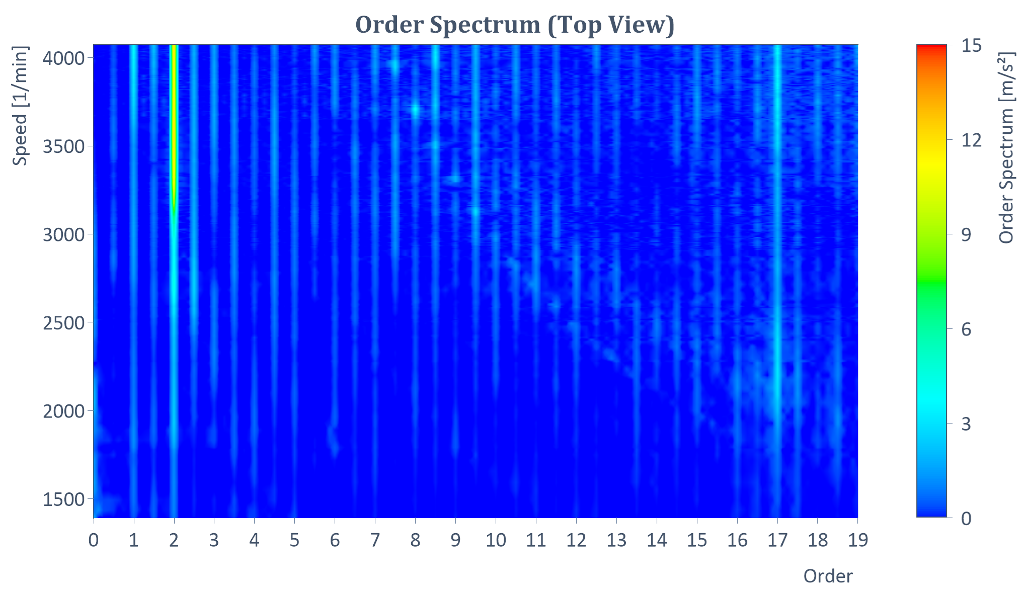
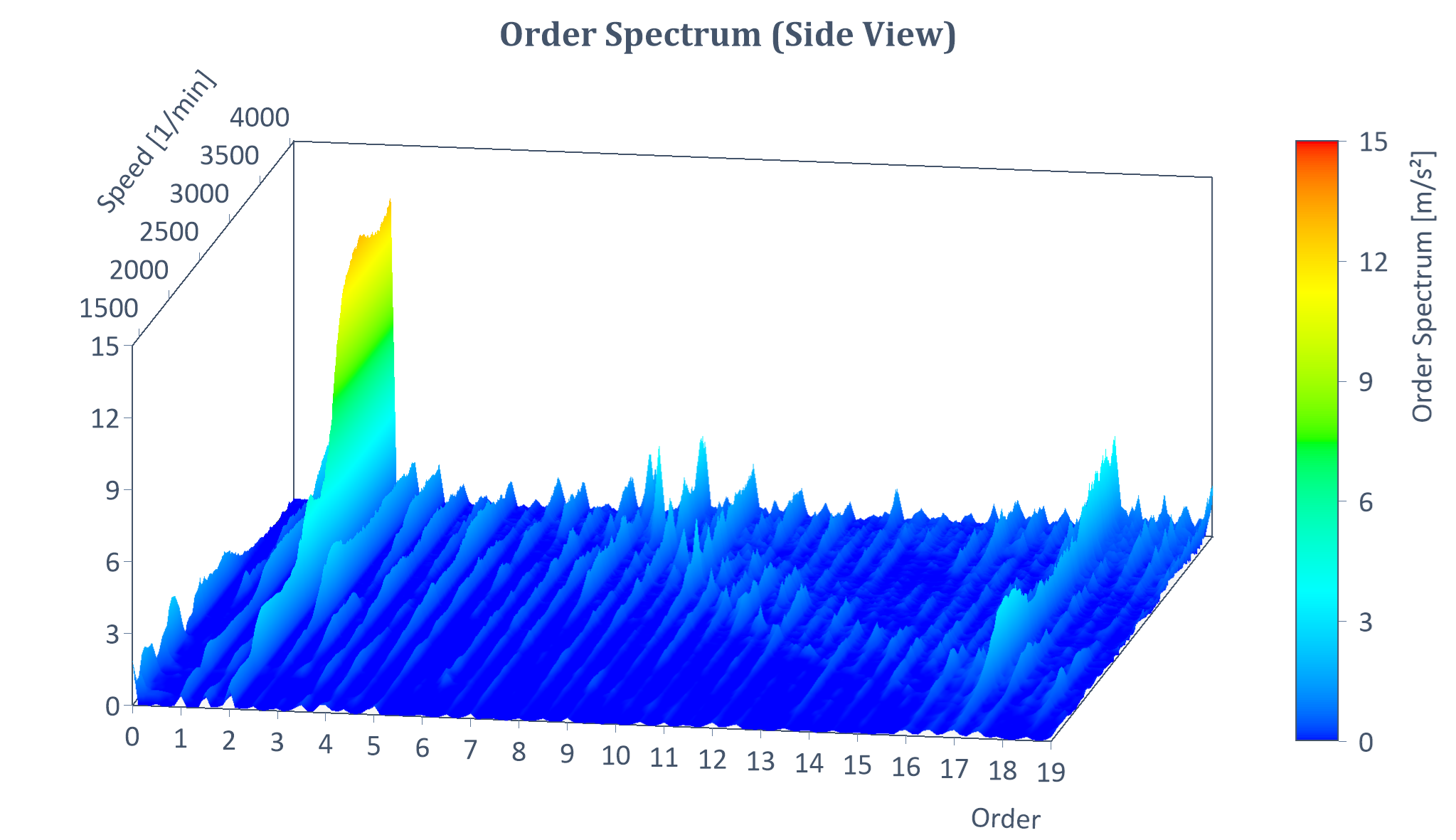
Example of an RMS order spectrum of a run-up (with Y = amplitude, X = order, Z = speed):
Result of the order cuts (as a list)
When selecting the output mode Extract orders from order spectrum (as a list), the following result types can be selected.
Result |
Description |
|---|---|
Y = amplitude, X = revolution |
List in which each element represents an order extracted from the order spectrum. The amplitude curves of the orders are each returned in each case across the revolutions. |
Y = amplitude, X = time |
List in which each element represents an order extracted from the order spectrum.The amplitude curves of the orders are returned in each case across the time. |
Y = amplitude, X = speed |
List in which each element represents an order extracted from the order spectrum. The amplitude curves of the orders are returned in each case across the rotational speed. It can be sorted monotonically in ascending order according to the speed. |
Y = amplitude, X = frequency (order * speed) |
List in which each element represents an order extracted from the order spectrum. The amplitude curves of the orders are each returned across the frequency (corresponds to product of order and speed). Resonance points are clearly visible in this illustration because they are now on top of each other. It can also be sorted monotonically in ascending order by speed. |
When calculating order cuts across the speed, the result contains non-equidistant speed sampling points (these correspond exactly to the equidistant revolution sampling points after calculation of the order spectrum in the revolution domain). The result can therefore also be evaluated across an equidistant speed range with the Speed start, Speed end and Speed increment to be defined. Here, linear interpolation is performed across the specified equidistant speed range. For linear resampling to produce meaningful results, the speed resolution calculated by the algorithm should be sufficiently high (e.g. the largest possible overlap in % of data segments and/or sufficiently small order resolution).
Result of the order cuts (as a signal series)
When selecting the output mode Extract orders from order spectrum (as a signal series), the following result types can be selected.
Result |
Description |
|---|---|
Y = amplitude, X = order, Z = revolution |
Signal series in which every signal contains the amplitudes of a particular revolution value across the extracted orders. |
Y = amplitude, Z = order, X = revolution |
Signal series in which each signal contains the amplitudes of an extracted order across the revolutions. |
Y = amplitude, X = order, Z = time |
Signal series in which each signal contains the amplitudes of a particular point in time across the extracted orders. |
Y = amplitude, Z = order, X = time |
Signal series in which each signal contains the amplitudes of an extracted order across time. |
Y = amplitude, X = order, Z = speed |
Signal series in which each signal contains the amplitudes of a particular rotational speed across the extracted orders. It can be sorted monotonically in ascending order according to the speed. |
Y = amplitude, Z = order, X = speed |
Signal series in which each signal contains the amplitudes of an extracted order across the speed. It can be sorted monotonically in ascending order according to the speed. |
Y = amplitude, X = order, Z = frequency (order * speed) |
Signal series in which each signal contains the amplitudes of an extracted order across the frequency (corresponds to the product of order and speed). Resonance points are clearly visible in this illustration because they are now on top of one another. It can also be sorted monotonically in ascending order by speed. |
Analogous to what was described before, the result can be evaluated when calculating Order cuts across the speed over an equidistant speed range.
Orders and bandwidths
If order cuts are calculated (or used to calculate the averaged RMS order cuts, see below), the orders to be analyzed can be explicitly set in a table or taken from a data set. The following three modes are available for extracting these orders from the order spectrum:
Extraction mode |
Description |
|---|---|
Order cuts without bandwidth |
The order curves (order cuts) are removed from the order spectrum without bandwidth. |
Order cuts as maximum in the order band |
The order curves (order cuts) are removed from the order spectrum as a maximum in the order band. |
Order cuts as RMS level in order band |
The order curves (order cuts) are removed from the power-normalized RMS order spectrum as an RMS level (energetically correct extraction). The spectrum type here in particular is always set to RMS and power normalization is always used. |
Note: Usually, the third mode, i.e. the energetically correct extraction by calculating the RMS level in the set order band, is used in most applications. This is the default setting for calculating the order cuts. The result clearly corresponds to the RMS curve of the signal bandpass filtered in the set order band. The same RMS curve of the respective order can therefore alternatively and equivalently also be calculated with the help of the Order Filter analysis object.
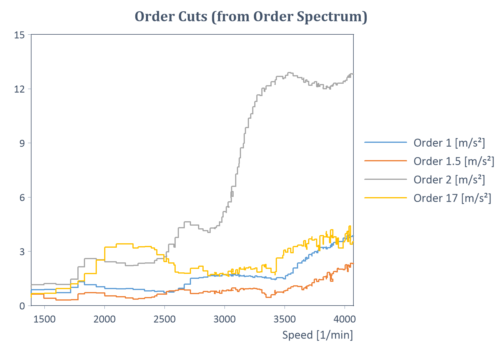
Example of RMS order cuts (as a list) of a run-up (with Y = amplitude, X = speed):
The result of averaged RMS order tracking
When selecting the output mode Averaged RMS order tracking, the following result types can be selected.
Result - Averaged RMS order tracking |
Description |
|---|---|
Averaged RMS order spectrum |
Calculates the arithmetic mean value in the RMS order spectrum for each order (spectrum type is always set to RMS here in particular). |
Averaged RMS order cuts |
Calculates the arithmetic mean of the RMS order cuts for each order (Spectrum type is always set to RMS, especially here, and power normalization is always used). |
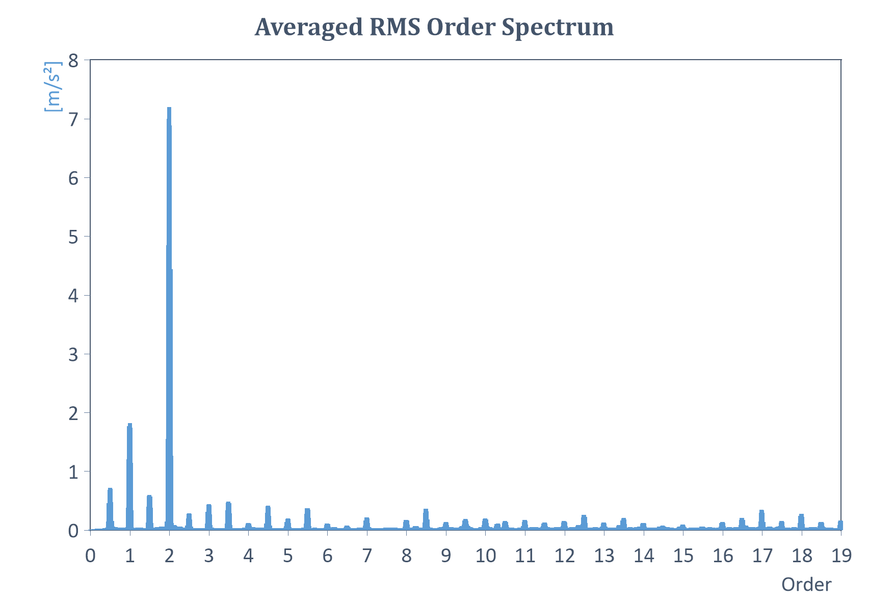
Example of an averaged RMS order spectrum of order tracking with constant speed:
Examples
In the project database C:\Users\Public\Documents\Weisang\FlexPro\2021\Examples\OrderT racking Analysis.fpd or C:>Users>Public>Public Documents>Weisang>FlexPro>2021\Examples\Order Tracking Analysis.fpd you will find examples of the different use cases and modes for which an order analysis can be performed. In particular, the diagrams above are included there.
FPScript Functions Used
See Also
Revolution Synchronous Sampling Analysis Object
You might be interested in these articles
You are currently viewing a placeholder content from Facebook. To access the actual content, click the button below. Please note that doing so will share data with third-party providers.
More InformationYou need to load content from reCAPTCHA to submit the form. Please note that doing so will share data with third-party providers.
More InformationYou are currently viewing a placeholder content from Instagram. To access the actual content, click the button below. Please note that doing so will share data with third-party providers.
More InformationYou are currently viewing a placeholder content from X. To access the actual content, click the button below. Please note that doing so will share data with third-party providers.
More Information