Continuous Wavelet Transform (CWT)
The Continuous Wavelet Transform (CWT) is used to decompose a signal into wavelets. Wavelets are small oscillations that are highly localized in time. While the Fourier Transform decomposes a signal into infinite length sines and cosines, effectively losing all time-localization information, the CWT's basis functions are scaled and shifted versions of the time-localized mother wavelet. The CWT is used to construct a time-frequency representation of a signal that offers very good time and frequency localization.
The CWT is an excellent tool for mapping the changing properties of non-stationary signals. The CWT is also an ideal tool for determining whether or not a signal is stationary in a global sense. When a signal is judged non-stationary, the CWT can be used to identify stationary sections of the data stream.
The core computations in FlexPro's CWT procedures generally follow the Torrence and Compo algorithms as listed in the references section below. The nomenclature that is used in the equations below also follows that used in the Torrence and Compo paper.
Continuous Wavelet Transform
The definitions for the CWT are as follows:
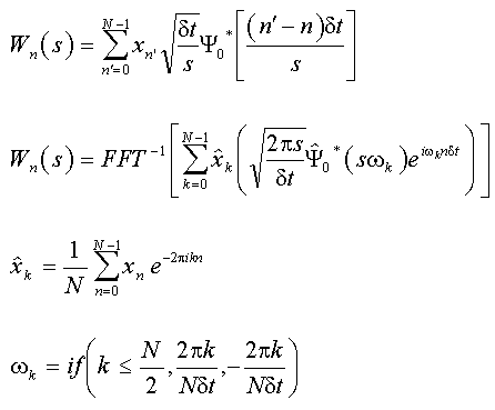
The CWT is a convolution of the data sequence with a scaled and translated version of the mother wavelet, the Ψ function. This convolution can be accomplished directly, as in the first equation, or via the FFT-based fast convolution in the second equation.
Note that the CWT is a continuous function except for the discrete data series x and its discrete Fourier transform. In these equations, * symbolizes a complex conjugation, N is the data series length, s is the wavelet scale, δt is the sampling interval, n is the localized time index, and ω is the angular frequency. Each of the equations contains a normalization so that the wavelet function contains unit energy at every scale.
In the CWT, for each value of the scale used, the correlation between the scaled wavelet and successive segments of the data stream is computed. Unless reconstruction is needed, there are no restrictions in the CWT as to how many scales are used, nor of the spacing between the scales. A CWT spectrum can use linear or logarithmic scales of any density desired. If needed, a high resolution spectrum can be generated for a narrow range of frequencies. The convolutions can be done up to N times at each scale, and must be done all N times if the FFT is used. The CWT consists of N spectral values for each scale used, each of these requiring an inverse FFT. The computational load of the CWT and its memory requirements are thus considerable. The benefit from this high measure of redundancy in the CWT is an accurate time-frequency spectrum.
Wavelet Basis Functions (Mother Wavelets)
Unlike a Fourier decomposition which always uses complex exponential (sine and cosine) basis functions, a wavelet decomposition uses a time-localized oscillatory function as the analyzing or mother wavelet. The mother wavelet is a function that is continuous in both time and frequency and serves as the source function from which scaled and translated basis functions are constructed. The mother wavelet can be complex or real, and it generally includes an adjustable parameter which controls the properties of the localized oscillation. Wavelet analysis is more complicated than Fourier analysis since one must fully specify the mother wavelet from which the basis functions will be constructed. FlexPro offers three different mother wavelets, each in complex and real-valued versions.
Morlet Wavelet
The most commonly used CWT wavelet is the Morlet wavelet, a Gaussian-windowed complex sinusoid that is defined as following in the time and frequency domains:
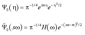
In these equations, η is a non-dimensional time parameter, m is the wavenumber, and H is the Heaviside function.
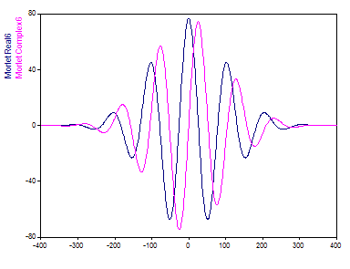
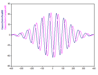
In the time domain plot that follows, the real and complex components of a Morlet wavelet with an adjustable parameter m (wavenumber) of 6 are shown:
The Morlet wavelet's adjustable parameter, the wavenumber, can vary from 6 to 100 in FlexPro. A Morlet wavelet with an adjustable parameter of 20 has a very different time domain representation:
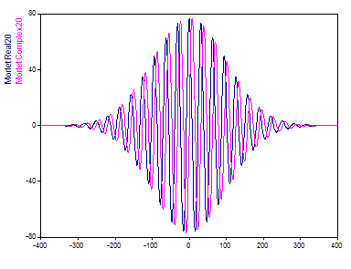
The number of oscillations in the Morlet wavelet is approximately that of the wavenumber.
Paul Wavelet
FlexPro also offers the Paul wavelet:
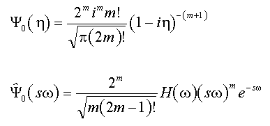
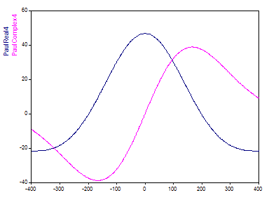
The Paul wavelet decays more quickly (as the square root of a factorial function). The Paul wavelet's adjustable parameter is an order that can vary from 4 to 40 within FlexPro. At an order of 4, only a single oscillation exists within the wavelet:
Even at the largest supported order of 40, the Paul wavelet evidences about the same oscillations than the Morlet at its lowest wavenumber:

The Paul wavelet offers better time localization than the Morlet because of its faster time-domain decay. Unlike the Morlet, however, its Fourier representation is not a symmetric peak but rather a peak that is right shifted toward higher frequencies. It approximately follows a gamma peak shape, and becomes less skewed as orders increase. Even at the Paul's highest supported order of 40, a significant right skew is evident in its frequency domain peak. The Paul wavelet thus offers poorer frequency resolution.
Derivative of Gaussian Wavelet
The third mother wavelet supported is the GaussDeriv (Gaussian Derivative). The real component is defined as follows:
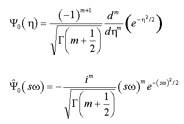
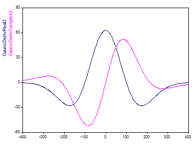
The complex wavelet is generated by the addition of a Heaviside function in the frequency domain. This wavelet decays with the square root of the gamma function. Its time localization is between that of the Morlet and Paul wavelets. The GaussDeriv wavelet's adjustable parameter is the derivative order that can vary from 2 to 80 within FlexPro. The lowest derivative, 2, is known as the Marr or Mexican Hat wavelet. A single oscillation is contained within the wavelet:
At its largest supported adjustable parameter of 80, the GaussDeriv wavelet contains about the same oscillation count as the Morlet with a wavenumber of 12:
Frequency Domain Representation
The frequency domain transform of the mother wavelets (Morlet wave number 6, Paul Wavelet order 40, and Gaussian Derivative order 20) is as follows:
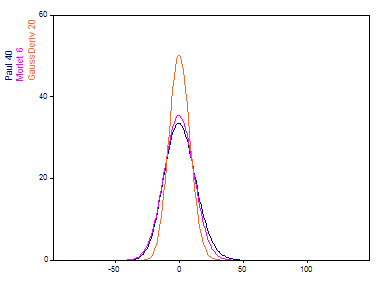
When the adjustable parameters for each of the three mother wavelets are set to produce approximately six oscillations, the Gaussian Derivative wavelet is shown to produce the most compact frequency domain spectral information. The Paul wavelet produces the least compact. The Morlet wavelet is between.
The Fourier transform of a Morlet wavelet produces a symmetric frequency domain peak. The GaussDeriv wavelet's frequency domain representation is exactly a gamma peak shape. The right shifted skew of the frequency peak is appreciably less than that of the Paul, and essentially vanishes above derivative order 20 or so (higher values for the derivative of the GaussDeriv wavelet produce nearly Gaussian frequency peaks).
Time Resolution vs. Frequency Resolution
All three of the wavelet bases are compactly supported, which means that the oscillations are effectively localized in time by rapid decays. For a given count of oscillations in the wavelet, the Paul wavelet localizes most efficiently in the time domain. The Morlet wavelet is slightly less efficient, and the Gaussian Derivative wavelet is the least efficient of the three. When comparing the frequency resolutions, however, the Gaussian Derivative wavelet is the best and the Paul wavelet is the poorest. The quality of the Morlet wavelet is in between.
While the Morlet wavelet is not as compact as the Gaussian Derivative for a given count of oscillations in the wavelet, it is capable of generating a much higher count of oscillations with the adjustment ranges supported in FlexPro. As such, a greater frequency resolution can be achieved using the Morlet wavelet.
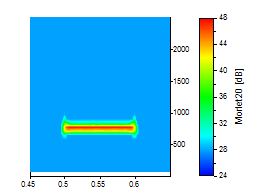
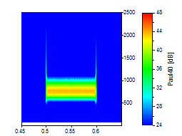
This can be better illustrated graphically. The following wavelet analyses use a noisy data set where a single sinusoidal oscillation occurs between 0.5 and 0.6 time:
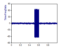
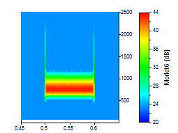
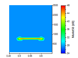
The wavelet peak has been zoomed in to illustrate this time-frequency resolution tradeoff. All plots use the same time-frequency scaling. The first three plots are for the Morlet at wavenumbers of 6, 20, and 50:
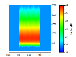
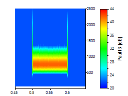
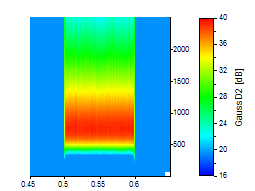
The next three are for the Paul wavelet at orders of 4, 16, and 40:
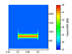
The final three are for the Gausssian Derivative wavelet at orders 2, 20, and 80:

In general, unless you need the best localization in time possible, the Morlet wavelet will probably suffice since it offers a very good resolution in both time and frequency.
Its frequency resolution is respectable even at the lowest wavenumber. The Paul wavelet's resolution in frequency at its best (order 40) is close to the Morlet with its least wavenumber of 6. You can also see the asymmetry in frequency in each of the Paul examples. If you need the best possible time localization, however, the Paul wavelet is a good choice.
The GaussDeriv wavelet at its best frequency resolution (order 80) is close to the Morlet with a wavenumber of 12. Unlike the Paul, higher orders of the GaussDeriv wavelet are essentially symmetric, and they can exceed the Morlet's frequency resolution with lower wavenumbers.
Multiresolution Analysis
For the Short-Time Fourier Transform , a fixed width segment size controls the time-frequency resolution tradeoff. This results in a single resolution in time and a single resolution in frequency, regardless of the frequency being rendered. In contrast, wavelet analysis is a multiresolution method. The time-frequency resolution is not constant, but varies with frequency. Multiresolution analysis was designed for the common condition where high frequency components exist for short durations within a signal, and low frequency components are more persistent.
Short-lived high frequency components need strong time localization. In order to achieve this, the frequency resolution of high frequency components will be diminished. On the other hand, long-lived low frequency components can tolerate poorer time resolution, but require effective frequency resolution. Low frequency components often determine the major part of a signal's character, and these properties will be best quantified if the frequency resolution is as fine as possible.
With multiresolution analysis, the difficult problem of determining an optimum segment width is avoided. The width of the time segments are automatically varied with frequency. The obvious drawback is that it is possible for a signal to contain short term low frequency components or long term high frequency components. For such signals, the Short Time Fourier Transform is probably a better choice than wavelet analysis. Furthermore, this variation in frequency resolution makes it impossible to read spectral powers or amplitudes directly from a wavelet spectrum. This is another instance where the single resolution analysis of the Short Time Fourier Transform may be preferable.
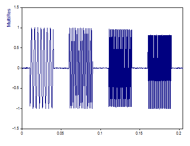
The following data set consists of sequential sinusoids of equal power in 1% white noise. Between times 0.01 and 0.04, a 250 frequency sinusoid is present. For times 0.06 to 0.09, a sinusoid is at 500 Hz frequency, for times 0.11 to 0.14, a 1000 Hz frequency sinusoid comprises the signal, and for times 0.16 to 0.19, a 2000 Hz frequency sinusoid is present.
In the CWT spectrum that follows, the Morlet wavelet with a wavenumber of 12 is used to generate a CWT spectrum:
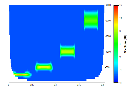
The multiresolution analysis is readily apparent. The 250 Hz frequency component is localized superbly in frequency, but is very fuzzy in time. Conversely the 2000 Hz frequency component is well defined in time, but quite fuzzy in frequency.
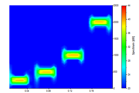
Contrast the CWT spectrum with an optimized STFT. The single resolution in the STFT is readily apparent:
Zero Padding and the Cone of Influence
The CWT spectrum is computed by first taking a discrete Fourier transform of the data series. Then for each scale (specified frequency) in the spectrum, the daughter wavelet's frequency response is analytically computed and it is multiplied by the data's frequency transform and an inverse is taken of the product.
Fourier transforms assume periodic data. For the FFT fast convolution to be free of wraparound effects that arise as a consequence of non-periodicity in both the data and the response function (daughter wavelet), zero padding is needed equal to the half the length of the non-zero elements in the daughter wavelet's frequency response.
This length will vary as a function of scale (frequency). Zero padding to twice the data size insures that no wraparound effects are possible anywhere in the spectrum. Often it is possible to zero pad to the next power of 2 and find negligible wraparound effects and achieve the fastest FFT performance.
When sufficient zero padding is used, the wraparound effect is eliminated but a different issue arises. By zero padding, it is likely that a discontinuity is introduced at the end of the data stream. Further, power is reduced near the edges of the spectrum with the introduction of the zeros into the convolution.
This zone of edge effects is known as the cone of influence (COI). In FlexPro, no spectral information in the zone of influence is shown. The spectral information within the cone of influence is not likely to be accurate regardless of whether or not zero padding is used. If it is not used, wraparound effects can occur at low frequencies. If it is used, the spectral powers may be diminished.
The cone of influence is computed using e-folding distances as per the Torrence and Compo reference.
Orthogonal Wavelets and the DWT
Most wavelet analysis uses a pair of filters to successively isolate low and high pass components of a signal. This is known as the Discrete Wavelet Transform (DWT). The DWT wavelets are not continuous functions of time and their transforms are not a continuous function of frequency. Rather they are sets of time-domain filter coefficients that generally produce an orthogonal basis that greatly simplifies data filtering and reconstruction. A DWT is non-redundant. The number of blocks of wavelet power at each scale is a function of non-overlapping wavelet width. In a typical DWT, frequencies are spaced at unit powers of two and the count of blocks in time will increase by unit powers of two as these fixed frequencies increase. Although the DWT is fast and its time-frequency representation of a signal requires only modest memory, it is not practical for time-frequency spectral analysis.
FlexPro exclusively uses the CWT for time-frequency spectral analysis. The CWT algorithms offer a greater accuracy, although this comes at a significant expense in computational load and memory usage.
References
For those who want to understand the subtleties of applying wavelet analysis to real-world data, there is a well-written paper that covers the CWT in a thorough and accessible manner:
•Christopher Torrence and Gilbert Compo, "A Practical Guide to Wavelet Analysis", Bulletin of the American Meteorological Society, v.79, no.1, p.61-78. January 1998
This reference explains the CWT in the context of analyzing El Nino time series data. The authors have also published a FORTRAN public domain CWT wavelet analysis package WAVEPACK. The WAVEPACK code is available on the Internet at: http://paos.colorado.edu/research/wavelets/
See Also
Time-Frequency Spectral Analysis Object - Continuous Wavelet Transform (CWT) Spectrum
You might be interested in these articles
You are currently viewing a placeholder content from Facebook. To access the actual content, click the button below. Please note that doing so will share data with third-party providers.
More InformationYou need to load content from reCAPTCHA to submit the form. Please note that doing so will share data with third-party providers.
More InformationYou are currently viewing a placeholder content from Instagram. To access the actual content, click the button below. Please note that doing so will share data with third-party providers.
More InformationYou are currently viewing a placeholder content from X. To access the actual content, click the button below. Please note that doing so will share data with third-party providers.
More Information