Non-Linear Curve Fitting Analysis Object and Template *
The Non-Linear Curve Fitting analysis object makes it possible to converge a model function dependent on an independent variable and several parameters toward a given data set. A number of pre-defined model functions are available to do this. Alternatively, you can define particular models.
Iterative and Non-Iterative Methods
For non-linear curve fitting methods, you can distinguish between iterative and non-iterative methods.
The non-iterative methods are generally not considered suitable, since they are very time intensive. This substantiates the "Grid Search" method. In this case, the range to be searched that contains the minimum is split into an n-dimensional (n... number of function parameters) grid. The residuals of the function are calculated for each grid point. The point at which the residual sum of squares is at its lowest returns the result. If the grid is then bisected, the number of function calls increases 2n times. With the "Random Search" method the points to be calculated are not assigned as grids, but are randomly distributed. The disadvantage of this method is that, as opposed to the iterative method, the search for the best parameters is not limited by the previous calculations. A number of "unnecessary" costly function calls are thus carried out.
Since using the iterative method does not guarantee that the calculated result is a "global minimum", it is suggested that you perform several calculations with different initial parameters. The non-iterative algorithms are useful for this.
In FlexPro, the FPScript function ParameterEstimation is therefore available to provide both the "Grid Search" method and the "Random Search" method. Due to the poor runtime response already described, the function is primarily suited for simple models with few parameters.
Among the iterative methods are the algorithms offered in the FPScript function NonLinearCurveFit , which gradually converge to a local minimum.
The following steps are carried out for this:
•The startup switches are determined for each parameter of the selected regression model (e.g. using the non-iterative methods).
•The curve is calculated in which the parameter values are implemented in the model function.
•The sum of squares of the vertical distances between data points and the curve is calculated.
•The parameters are modified in such a way that the curve converges better to the data points. Various algorithms are used for this.
•The steps 1 to 4 are repeated as long as a "good" result is achieved. There are various convergence criteria that can be set for this.
A search is thus performed for the parameters of a model, which minimizes the weighted residual sum of squares as much as possible and thereby provides a suitable convergence to a given data set.

Vectors with parameter values are calculated from a given start point on, which converge on a local minimum. The different methods are distinguished by the calculation of the increment, the direction of the increment and the convergence criteria.
The applied algorithms form the following methods:
Gauss-Newton Method
For the Gauss-Newton method, the model is linearized using Taylor expansion. The linearized model is then used to minimize the residual sum of squares.
Steepest Descent Method
When searching for the minimum, the direction of descent is specified by the (negative) function gradients.
Thus, the method is also called the gradient method. As a rule, it finds the optimum rather slowly, meaning that it converges poorly.
Levenberg-Marquardt Method
The Levenberg-Marquardt method combines the Gauss-Newton method with the steepest descent method. The "Trust Region" radius used for the method influences the increment and increment direction. It provides an upper bound for the Euclidean norm of the search direction and thus influences the method used (Gauss-Newton or steepest descent).
Newton Method
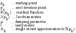
Contrary to the Gauss-Newton method, this method examines the square part of the Taylor expansion. Thus, the Hessian matrix (second partial derivatives) is required for the calculation. Since the Hessian matrix can rarely be specified analytically, it must be approximated. This occurs, for instance via the secant method. Good algorithms replace the Hessian matrix so that information that is already available can be used and thus you obtain a better approximation. Instead of H(x), only S(x) is approximated:
Hessian Matrix:
![]()
Calculating the next iteration p+ from one point pk:
Methods |
Calculated Using |
|---|---|
Gauss-Newton |
|
Levenberg-Marquardt |
|
Newton |
|
NL2SOL |
|
Algorithms
For algorithms used in non-linear curve fitting, a Moré procedure in a MINPACK package (Levenberg Marquardt algorithm) and a variant of the NL2SOL algorithm (Full Newton algorithm). In the References section, both algorithms can be found that are almost of equal value. There is no great difference for problems with small residuals. The more complex NL2SOL algorithm is, however, preferred for problems with larger residuals or for extremely non-linear problems, since it requires fewer iterations. In addition, bounds for the parameters to be found are kept when implementing variations of the NL2SOL algorithm and thus the range to be searched is limited. Both algorithms were already tested thoroughly for applicability and robustness.
For both algorithms, the partial derivatives that are required for the calculation can be calculated analytically as well as "approximated through forward-difference approximation". When calculated analytically, the partial derivatives are specified as formulas. This is the case for almost all given models. If the derivatives are not specified for a custom model, they are approximated.
A modified Levenberg-Marquardt algorithm is used for the algorithm LMDER or LMDIF in MINPACK. Moré uses a scaled "Trust Region" method.
The NL2SOL algorithm is based on the Newton method of "least squares". It contains a secant method for calculating the Hessian matrix. In addition, a "trust region" strategy is used. For problems with small residuals, the algorithm is simplified to a Levenberg-Marquardt or a Gauss-Newton method. Both algorithms can be found on the Internet under www.netlib.org.
Model
FlexPro offers a variety of pre-defined model functionsto which the data to be analyzed can be adapted. After you have selected a model, you can view the formula and a sketch of the associated model in a preview pane. You can access FlexPro Online Help for the model functions directly using the Help on Models button. The current model function can be viewed, for instance, while you are setting the initial values of the parameters so that you do not have to switch between tabs.
Peak Models
A number of pre-defined peak models are available that can be modified using the number of peaks and the information for a baseline function. For models with several peaks, certain model parameters can be used together. This can be set up in the parameters list . Using this information, a "special" peak model is generated dynamically and used for non-linear curve fitting. FlexPro offers peak fitting in the Analysis Wizard as a separate analysis template.
Custom Model
If the model to be analyzed is not found in the list of pre-defined model functions, a custom model can be defined and stored in the user profile. To do this, you first have to select the model (custom model). The Function text box appears where the custom model is entered. The parameters of a custom model with a number of parameters of n are named p[0], p[1], ..., p[n-1]. The independent variable is x.
Example of a sine function: p[0] * sin(2 * PI * p[1] * x + p[2])
You can also assign the parameters names. These names then appear in the Initial Values list. To do this, you must assign names to the parameter variables p[0] … p[n-1] in the formula that describes the custom model function.
Dim Amplitude = p[0]
Dim Frequency = p[1]
Dim Phase = p[2]
The Amplitude variable is assigned to the variable p[0], Frequency is assigned to p[1], and Phase is assigned to p[2]. You must make sure that the assignments are made one below another. In the model function, you can now replace the variables p[0] through p[n-1]:
Amplitude * sin(2 * PI * Frequency * x + Phase)
When defining a custom model, it is important to enter the correct Parameter count. If this value is wrong, non-linear curve fitting cannot be calculated or will return an incorrect result.
•Calculate partial derivatives analytically
The algorithms for non-linear curve fitting require the partial derivatives of the model parameters for the calculation. The derivatives can be calculated analytically as well as through "forward-difference approximation". When calculated analytically, the partial derivatives are specified as formulas. The formula that describes the derivatives must be specified as a List with n (number of parameters) derivative functions.
Example:
Dim Amplitude = p[0]
Dim Frequency = p[1]
Dim Phase = p[2]
[ sin(2 * PI * Frequency * x + Phase), 2 * PI * x * Amplitude * cos(2 * PI * Frequency * x + Phase), Amplitude * cos(2 * PI * Frequency * x + Phase) ]
•Save Model
You can save a custom model in your User profile. To do this, you must enter a name in the Model list box and press Save Model. All saved models appear in the Model list box. If you select a custom model, you can delete it from the user profile by pressing the Delete Model button.
•Custom model from formula
You can also save database-dependent custom models by setting up formulas with the model functions. To do this, you have to select the (Custom model from formula) model and specify the model formula generated as the function. The syntax for the model formulas is described under Custom Model. However, the content of the formula must be placed in quotation marks, since the model formulas must be of the string data type.
The formula for the above model should be look like the following:
"Dim Amplitude = p[0]\r\n_
Dim Frequency = p[1]\r\n_
Dim Phase = p[2]\r\n_
Amplitude * sin(2 * PI * Frequency * x + Phase)"
The formula for the partial derivatives must contain the following code:
"Dim Amplitude = p[0]\r\n_
Dim Frequency = p[1]\r\n_
Dim Phase = p[2]\r\n_
[ sin(2 * PI * Frequency * x + Phase),_
2 * PI * x * Amplitude * cos(2 * PI * Frequency * x + Phase),_
Amplitude * cos(2 * PI * Frequency * x + Phase) ]"
The "\r\n" characters generate a line break in a string and must be used if your code contains multiple statements. In this example, the character "_" was used at the ends of lines so that the string could be split across several lines.
Model Ranking (only in Analysis Wizard)
With this tool, you can compare the calculation of several model functions to one another. The ranking of the selected models occurs via the absolute residual sum of squares SSE. For more information on this, refer to the Non-Linear Curve Fitting Tutorial.
Parameters
Selecting the initial values of the model parameters is decisive in calculating the result. If the selected starting point is far away from the global minimum, the algorithm may not return a result or may return a different local minimum. For the Full Newton algorithm, a range limit (upper and lower bounds) is specified for each parameter, thereby narrowing range of the search.
Certain parameters of the selected model can be declared as fixed. For the Full Newton algorithm, the upper and lower limits are set to the specified initial value. For the Levenberg-Marquardt algorithm, the parameter variable in the model function is replaced by the constant initial value.
Estimate Initial Values (only in Analysis Wizard)
To increase the probability that a global minimum is in the result displayed, the calculation should be carried out with different initial values. For models with four or fewer parameters, the Estimate Initial Parameters . For each parameter, 10 randomly distributed values are calculated that are found in the range determined by the upper and lower bounds. For each combination, the absolute residual sum of squares is now calculated. The combination with the least square mean sum provides the initial values.
Start Script
The initial parameter values can also be calculated using an FPScript formula. When you do this, make sure that the result of the formula returns a data series with n (number of model parameters) values. Otherwise, the Start Script is ignored. To edit the formula, click on the Start Script. You can edit the code in the dialog box that appears. Use the data variable to access the data. You can use the Calculate button. By clicking Apply, you are accepting the calculated parameters. Additionally, in the Analysis Wizard you can select the option Use start script. The start script is then automatically calculated whenever the model is changed or when non-linear curve fitting is called up again.
Weighting
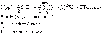
Determining the best parameter using minimization of the residual sum of squares is based on the assumption that the scattering of values is equal to the determined curve of a Gaussian distribution. The lease mean square error method is an estimate of maximum likelihood if the errors of measurement are independent and normally distributed (Gaussian distribution) and have a constant standard deviation. Measured values that are further from the given curve influence the residual sum of squares more strongly than closer points.
If the scattering for all data points is the same, then no weighting is necessary. The weighting vector W is 1 for each parameter.
There are also experimental situations where the distance of the residuals increases as Y increases. If the absolute spacing of the curve points increases as Y increases, but the relative spacing (spacing divided by Y) remains constant, a relative weighting of W = 1/Y2 makes sense. Thus, the sum of square of distances is:
![]()
The Poisson weighting of W = 1/Y represents a compromise between the minimization of the relative and absolute distance. For a Poisson distribution, the following is especially important:
![]()
In addition, the residual sum of squares can be weighted with the variance. If the data to be examined are specified as a data matrix or a data series, the variance s2 with the setting "Weighting with 1/s2, 1/s2 is determined from the data matrix" over the data and is used as weighting:
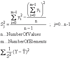
The variance s2 is then specified via a data set. The data length of the variance must equal the data length of the data set to be examined.
Scaling
One problem for non-linear curve fitting can be the poor scaling of individual model parameters. For instance, a variable could move in a range of [102, 103] meters and another in an interval of [10-7, 10-6] seconds. If this point is ignored, then this can have a negative influence on the calculated results.
Consequently, for the respective algorithms, different scaling options (No Scaling, Adaptive Scaling, Scaling From Initial Jacobian Matrix, Scaling From Bounds, Custom Scaling) are available. In the example provided, you could select a custom scaling and recalculate the first parameter in kilometers and the second parameter in milliseconds. Both parameters then lie within the interval [10-1,1]. In addition to influencing the algorithm, the scaling plays an important role in calculating diverse convergence criteria. When calculating without scaling, the parameters with a very small range of values are ignored when testing convergence criteria.
Termination Criteria and Settings
It is important to know when calculating parameters how you should terminate the algorithm. The issue is when can a calculation be completed successfully and when is it time to abort the calculation with an error message.
There are a variety of convergence criteria that determine whether the currently calculated parameters are close enough to the desired solution that the calculation can be completed. The convergence tolerances can be set via the parameters X Tolerance, Y Tolerance, F Tolerance or G Tolerance. The calculation of convergence criteria is differentiated through the algorithms.
•The NL2SOL algorithm 5 convergence tests:
- X convergence (relative parameter convergence criterion)
- relative function convergence
- absolute function convergence
- singular convergence
- false convergence
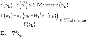
The first three convergence criteria can be influenced by the X Tolerance, Y Tolerance and F-Tolerance settings options. The Absolute Function Convergence occurs when a pk iteration is found where it applies for a given F-Tolerance tolerance.
The other convergence criteria are then only carried out if the current step Δpk leads to no more than twice the predicted function reduction:
![]()
The convergence tests are strongly influenced by the current square model qk, which is quite unreliable, if the inequality specified is not fulfilled. This test therefore offers extra protection with regard to the reliability of the other convergence criteria.
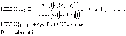
X Convergence (XTolerance) tests the relative scaled parameter changes per iteration step:
The Relative Function Convergence (YTolerance) is obtained when the function with the current calculated parameters lies near an estimated function f(p*) with a strong local minimizer p*. The estimated function converges via a square model:
•Minpack:
The Relative Parameter Convergence (X Convergence) is based on the relationship of the absolute parameter change to the relative change of the Euclidian norm of the parameter. This convergence criterion can be influenced by the X Tolerance parameter.
To test the relative function convergence, the MINPACK algorithm LMDER or LMDIF calculates the current relative change in the sum of squares during one iteration and the estimated relative change based on a linear model. The convergence criterion is fulfilled when both relative changes are less than the given Y Tolerance tolerance.
With the G-Tolerance parameter, you determine how large the cosine of the angle between the columns of the current Jacobian matrix and the corresponding residual vector is allowed to be. The orthogonality can thus be determined. A mathematical relationship between this test and the test for relative parameter convergence in the NL2SOL algorithm can be produced (compare to Dennis: An Adaptive Non-Linear Least Square Algorithm).
In addition, you can specify the maximum number of times the function can be called to calculate the residuals before the calculation is terminated. It is possible that the residual function could be called several times per iteration step. You should therefore not specify the maximum number of iterations, but instead specify the minimum number of function calls.
The initial step length can be changed using Step bound. This must be changed in situations where you want to prevent the first step from being too large, which, for instance, leads to an exponential overflow. The diameter of the "trust region" is determined, in which the best parameters can be searched for during the first iteration.
Result / Output (only in the analysis object)
The Status output describes the reason why a calculation was aborted. A distinction is made between two groups. The algorithm ends successfully if certain convergence criteria are fulfilled. If this is not the case, the algorithm aborts the calculation based on termination criteria. The convergence criteria alone, however, are not sufficient to determine the result of the non-linear curve fitting. Different statistical output options are therefore available with which the grade of the fit can be determined.
The non-linear curve fitting provides you with two output alternatives. You can calculate the parameters once and enter them statically into the selected model function. For this, use the NonLinModel function for the pre-defined models. To generate a static model, you need to press the Calculate Curve Fit button. The calculated values will appear in the parameters list. Alternatively, you can determine in the Output tab which statistical characteristic quantities are to be output. If several output options are selected, the analysis object returns a list as the result. (See NonLinearCurveFit)
References
•P.R. Bevington, D.K. Robinson. Data Reduction and Error Analysis for the Physical Sciences, 3rd Ed., McGraw-Hill, New York, 2003.
•W. H. Press, S. A. Teukolsky, W. T. Vetterling, B. P. Flannery. Numerical Recipes in C. 2nd ed. Cambridge, U.K., Cambridge Univ. Press, 1992.
•G. A. F. Seber, C. J. Wild. Nonlinear Regression. Wiley, New York, 2003.
•K. Madsen, H.B. Nielsen, O. Tingleff, Methods for non-linear least squares problems, 2nd Edition, IMM, DTU, April 2004
•P.E. Frandsen, K. Jonasson, H. B.Nielsen. Unconstrained Optimization, 3nd Edition, IMM, DTU, March 2004
•Harvey Motulsky, Arthur Christopoulos. Fitting Models to Biological Data Using Linear and Nonlinear Regression: A Practical Guide to Curve Fitting. Oxford University Press, 2004.
You can find information on the algorithms here:
•J. E. Dennis Jr., Robert B. Schnabel. Numerical Methods for Unconstrained Optimization and Nonlinear Equations. Classics in Applied Mathematics 16, SIAM Society for Industrial and Applied Mathematics, 1996.
•J. E. Dennis, Jr., D. M. Gay, and R. E. Welsch. An Adaptive Nonlinear Least Square Algorithm, ACM Trans. Math. Software 7, 1981, pp. 348-368 and 369-383
•J. E. Dennis, Jr., D. M. Gay, and R. E. Welsch. Algorithm 573. NL2SOL -- An adaptive nonlinear least-squares algorithm, ACM Trans. Math. Software 7, 1981, pp. 369-383.
•D.W. Marquardt. An Algorithm for Least-Squares Estimation of Nonlinear Parameters, Journal of the Society for Industrial and Applied Mathematics, vol. 11, 1963, pp 431-441.
•Jorge J. Moré. The Levenberg-Marquardt Algorithm: Implementation and Theory, Numerical Analysis, Lecture Notes in Mathematics, vol. 630, G.A. Watson, ed. (Berlin: Springer Verlag), 1977, pp. 105- 116.
•J. J. Moré, B. S. Garbow, and K. E. Hillstrom. User Guide for MINPACK-1, Argonne National Laboratory Report ANL-80-74, Argonne, Ill., 1980. Internet: http://www.netlib.org/minpack/ex/file06
•P. A. Fox, A. D. Hall, and N. L. Schryer. The PORT mathematical subroutine library, ACM Trans. Math. Software 4, 1978, pp. 104-126.
•D. M. Gay. Usage summary for selected optimization routines, Computing Science Technical Report No. 153, AT\&T Bell Laboratories, Murray Hill, NJ, 1990.
•K.L. Hierbert. An Evaluation of Mathematical Software that Solves Nonlinear Least Squares Problems. ACM Trans. Math. Software, Vol. 7, No. 1, 1981, pp. 1-16.
FPScript Functions Used
See Also
Non-Linear Curve Fitting Tutorial
Statistical Output Options for Non-Linear Curve Fitting
* This analysis object is not available in FlexPro View.
You might be interested in these articles
You are currently viewing a placeholder content from Facebook. To access the actual content, click the button below. Please note that doing so will share data with third-party providers.
More InformationYou need to load content from reCAPTCHA to submit the form. Please note that doing so will share data with third-party providers.
More InformationYou are currently viewing a placeholder content from Instagram. To access the actual content, click the button below. Please note that doing so will share data with third-party providers.
More InformationYou are currently viewing a placeholder content from X. To access the actual content, click the button below. Please note that doing so will share data with third-party providers.
More Information