This tutorial covers the spectral analysis capabilities of FlexPro that rely on autoregressive parametric modeling and eigenanalysis procedures. These advanced procedures are particularly important for frequency estimation when data records are very short.
Frequency Estimators
The AR and ARMA spectral estimators are modeling procedures that use an autoregressive (AR) or autoregressive-moving average (ARMA) model to estimate the spectra of time domain data. Eigenanalysis uses the noise eigenmodes to reconstruct an orthogonal frequency spectrum that contains only the narrowband signal components. All three algorithms are spectral estimators, i.e. they provide a very accurate estimate of the frequencies of existing harmonics. However, these procedures do not generally yield an accurate measure of power in the components.
Extracting Stationary Segments
Because these methods are computationally intense, they are most useful for small data sets where Fourier analysis lacks sufficient resolution. Also, since signal data are assumed stationary, it is sometimes useful to extract a small segment of a data stream where the signal can be assumed to be approximately stationary (unchanging its overall spectral content). In this tutorial, we will use a small data length test sample that could easily be a small piece within a much larger sample.
A Suitable Test Signal
For this tutorial, we will use a short 64-length data signal that contains three sinusoids spaced too closely in frequency to be resolved by Fourier analysis.
100.0*sin(2π*x*420+π/2)
50.0*sin(2π*x*500+π)
100.0*sin(2π*x*580+3π/2)
The sample rate is 5000 Hz, and as such the Nyquist frequency is 2500 KHz, the maximum frequency that can be detected. Any oscillatory information beyond this frequency will be aliased to lower frequencies. The time values vary from 0 to 0.0126 with a sampling interval of 0.0002. 10 % random Gaussian noise was added to both signals. This produces a noise floor at about -30 dB relative to the largest peak.
The middle sinusoid has half-amplitude or one-quarter power of the other two sinusoids. Note that is not a high dynamic range test, but one where all three peaks have substantial power. This middle peak is only -6 dB below the other two peaks. As such, the optimizations in the Fourier domain will have little impact on resolving this one-quarter power center peak.
Select the command File > Open Project Database and open the project database C:\Users\Public\Documents\Weisang\FlexPro\2025\Examples\Tutorials\Spectral Analysis.fpd or C:>Users>Public>Public Documents>Weisang>FlexPro>2025>Examples>Tutorials>Spectral Analysis.fpd. Open the Tutorials folder and its Frequency Estimators subfolder and then double-click to open the 2D diagram called Data.
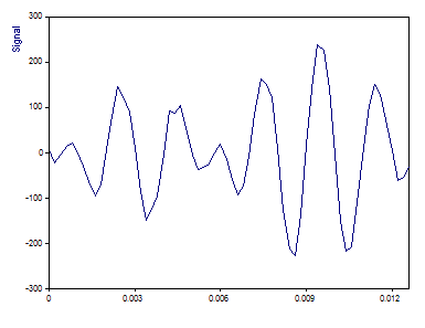
This is a graph of the signal. There are 64 floating point values.
Fourier Spectrum
We will use a Hamming data taper to realize the maximum side lobe damping for a one sided Fourier width of 2.
Close the graph window and highlight the Signal data set.
Click on Insert[Analyses] > Analysis Wizard.
Select the Fourier Analysis category under Spectral Analyses. Next, select Fourier Spectrum. Click on Next.
Note that for Spectral Procedure, the Fourier Spectrum is checked. Although the Spectral Procedure was selected in Step 1 of the Analysis Wizard, this can be modified in Step 2.
Select for the Spectrum Type the value dB normalized.
This normalizes the largest spectral peak to 0 dB. All other peaks will have a negative value. A peak at -3 dB would have half the power of the 0 dB peak, and a peak at -6 dB would have half the amplitude, the value expected for the middle of the three peaks.
For the Window Type select Hamming -43 dB W=2.
In FlexPro's Spectral Analysis module, all fixed width (non-adjustable) data tapers are listed by their names, the side lobe attenuation in dB, and the one-sided Fourier domain peak width. A rectangular window is the same as no windowing, as all data elements are multiplied by unity.
Make sure that the FFT length is set to data length or 64.
The Zero Pad informational field shows that no zero padding has taken place.
Select the Maximum peak count option and enter the value 3.
The Analysis Wizard automatically generates spectral peak information. With this option set to 3, the three peaks of highest power will be output. Note that it is also possible to set a dB threshold below the largest peak. For this data set, we could have as easily set a -65 dB threshold.
Now set the White Noise Critical Limit % to None.
If no labels are visible above the peaks, click on Toggle Labels until the frequency labels appear.
You can choose from several settings. You can switch on the labelling for the Y component of the spectrum (here in dB, normalized) or for the X component (always frequencies). Alternatively, you can also switch off the labelling.
The Fourier plot in the Analysis Wizard should be as follows:
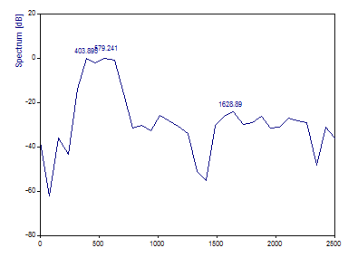
Set the FFT length to 8192.
The interpolation introduced by zero padding causes the 420 and 580 highest power peaks are more accurately resolved, but the sample length is too small to produce any resolution of the lower amplitude sinusoid with frequency 500. Nothing can be done to bring the needed resolution to the Fourier analysis of this particular data sample. What is needed is to sample for a longer time. We will see what happens when this same data stream is sampled for twice as long.
Click on Cancel. Select the Signal2 data set.
Again, select the Analysis Wizard. Select the Fourier Analysis category under Spectral Analyses. Next, select Fourier Spectrum. Click on Next. Set the Spectrum Type to dB normalized, the Window Type to Hamming -43 dB W=2. Set the FFT length to 8192, Maximum peak count to 3, White Noise Critical Limit % to None. If no labels are visible above the peaks, click on Toggle Labels until the frequency labels appear.
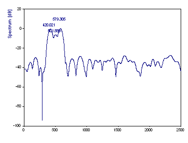
The 420 Hz component is detected at 420.02, the 500 Hz component at 501.89 and the 580 Hz component at 579.30. The third peak has the highest power and is therefore 0 dB. The first peak was -0.21 dB, the middle peak -6.20 dB.
At this sample length, there is sufficient Fourier resolution to resolve the three components. Note that despite being on the borderline of resolution, the accuracy in both frequency and power estimates is very good. The purpose of this exercise is to illustrate the merit in thoroughly exploring the Fourier approach before turning to alternative procedures.
What happens, though, when it is not possible to increase the information in the data by sampling for a greater length of time? If the data is an approximately stationary snapshot taken from a rapidly changing signal, it may not be possible to increase the frequency resolution by using a longer sample. In cases such as these, the parametric AR and ARMA and the Eigenanalysis procedures are needed.
AR Estimation Spectra
The frequency estimation methods that we will now explore are powerful methods when the data length is too short for sufficient Fourier analysis resolution.
Click on Cancel. Highlight the originally used data set Signal. This will have 64 data elements.
Again, select the Analysis Wizard. Select the Spectral Estimator category under Spectral Analyses. Next, select AR Spectral Estimator. Click on Next.
Select the algorithm Data matrix FB SVD.
The Autocorrelation, Burg, Normal Equations FB and Data Matrix FB procedures do not offer integrated separation of signal and noise. They are offered in FlexPro for comparative analysis and because these procedures have been historically used for AR analyses. These procedures can produce spurious peaks, split peaks, and other anomalies that are dangerous in spectral analysis. Therefore, only the two algorithms Normal Equations FB SVD and Data Matrix FB SVD are recommended.
The procedure Normal Equations FB SVD can be used to reduce the calculation time. It is much faster than the Data Matrix FB SVD procedure on very long data sets.
Set the Spectrum type to dB, the Order to 40 and the Signal Subspace to 6.
The order of 40 means that an AR model of 40 coefficients will be generated. A signal space of 6 means that only 6 of the eigenmodes will be treated as signal. The other 34 eigenmodes will be treated as noise and discarded in the SVD computation of the AR coefficients. The intrinsic signal-noise separation eliminates the influence of noise on the spectrum.
Please note that you must increase the signal subspace by 2 for each additional spectral component. For example, to map three spectral components, the signal subspace must be set to double, i.e. 6. Please also note that for these procedures, no maximum number of peaks needs to be specified for labeling the peaks in the spectrum. For the non-SVD algorithms, this number results from the number of roots of the AR polynomial and for the algorithms with SVD from the size of the signal subspace.
Select the Adaptive spacing option.
The Adaptive spacing option furnishes a full frequency range spectrum that is adaptive. The frequency values are then close together in the area of sharp peaks and further apart at the points where the spectral amplitude is subject to smaller changes.
If no labels are visible above the peaks, click on Toggle Labels until the frequency labels appear.
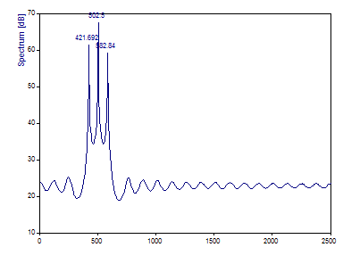
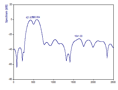
While nothing could be done with Fourier analysis to resolve the intermediate frequency harmonic, a properly designed AR spectral analysis clearly recovers the three spectral components. The very sharp spectral peaks are typical of harmonics in AR spectra.
The 420 Hz component is estimated at 421.69, the 500 Hz component at 502.5 and the 580 Hz component at 582.84. Although the comparison with the Fourier spectra of the same data (with 64 points) is impressive, the Fourier analysis would provide a more accurate frequency estimate with a data length of 128. Note also that the magnitudes of the AR peaks are the reverse of the power or amplitude profile. The middle component is shown to have the highest magnitude in the spectrum. This is why the AR method should be regarded primarily as a frequency estimator only. Again, the two step procedure in the Harmonic Analysis option should be used to estimate amplitudes and powers of components.
Now select the Data Matrix FB algorithm.
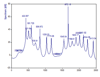
This is more what conventional AR spectral analysis has yielded historically, and why it has a poor reputation in many circles. Unless there is intrinsic signal-noise separation in the AR coefficient computations, an AR model will typically produce the half the model order in peaks, and it is not uncommon for some of these to be spurious. A noise peak is shown to have a spectral magnitude greater than that of the three target peaks.
Select the Autocorrelation method.
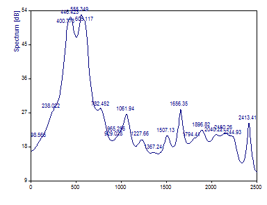
Because the AR filters of this procedure are always stable (the complex roots of the AR polynomial always lie in or on the unit circle), the disturbing peaks of the other ordinary AR algorithm without singular value decomposition appear less frequently. But this method has a significantly poorer frequency resolution. Note that this AR method is unable to resolve the middle component.
Eigenanalysis Spectra
The eigenanalysis methods are generally regarded as the most accurate class of frequency estimators. The MUSIC (MUltiple SIgnal Classification) and Eigenvector algorithms are in widespread use for accurately estimating narrowband components within signals.
Select the Spectral Procedure Eigen (MUSIC, EV) and for the algorithm MUSIC. Make sure that the Spectrum Type is set to dB, the Order is set to 40 and Signal Subspace is at 6. Retain the Adaptive spacing option.
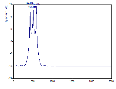
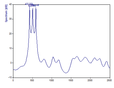
The 420 Hz component is estimated at 422.32, the 500 Hz component at 501.56 and the 580 Hz component at 583.77. Although the comparison with the Fourier spectra of the same data (with 64 points) is impressive, the Fourier analysis with a data length of 128 would also provide a more accurate frequency estimate here.
Further, these estimates are not quite as accurate as the AR procedure. Here, though, the middle component is shown to have a lower magnitude in the spectrum. While the correct profile in this instance, the Eigenanalysis methods are likewise to be regarded only as frequency estimators. Again, the two step procedure in the Harmonic Analysis option should be used to estimate amplitudes and powers of components.
Select the EV (EigenVector) algorithm.
The 420 Hz component is estimated at 422.30 Hz, the 500 Hz component at 502.55 and the 580 Hz component at 584.14. For these data, the MUSIC procedure was slightly better at estimating the frequencies.
In these procedures, noise eigenmodes are used to generate the signal spectra. There should therefore always be a high number of noise eigenmodes in order to adequately map the noise in the signal. The difference between the MUSIC and EV algorithms is only in how the different noise eigenmodes are weighted.
Harmonic Estimation
We will now employ a two-stage harmonic analysis to extract the amplitudes and power of the spectral components.
Click on the Back button. Select the Harmonic Analyses and then select Harmonic Estimation. Click on Next.
Select the AR Data Matrix FB SVD algorithm, set the Number of Components to By maximum count. Set the Maximum count to 3 and the Spectrum Type to Harmonic Components. Set the Order to 32.
A lower order must be specified in this two-step procedure. Anomalies can occur if the model order is pushed above 1/2 the data length. To safeguard against these effects which are not readily observed in this automated two-step algorithm, FlexPro limits the model orders in the Harmonic Spectrum to 1/2 the data length.
Click on Toggle Labels until the amplitude labels appear.
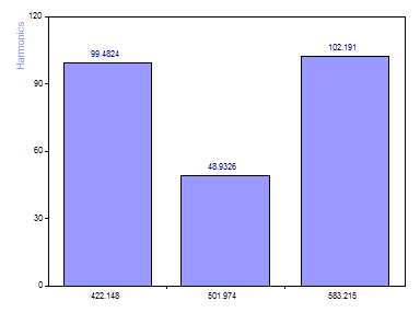
Note that the [100, 50, 100] amplitudes are recovered to within a few percent.
Click on Next. Select all objects in step 3 and click Finish.
Double-click on the object HarmonicEstimation in FlexPro's Object List.
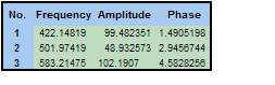
The phases used in the original signal are π/2, π,3π/2. It is typical that the smallest errors occur in the frequencies and the largest errors in the phases. Here the 1.57 phase is 1.49, the 3.14 phase is 2.94 and the 4.71 phase is 4.58. These are still very good values when you consider that a full 10 % noise was added to the test signal.
References
Excellent coverage of AR spectral algorithms can be found in the following references:
•S. Lawrence Marple, Jr., "Digital Spectral Analysis with Applications", Prentice-Hall, 1987, p.172-284.
•Steven M. Kay, "Modern Spectral Estimation", Prentice Hall, 1988, p.153-270.
Also of interest may be the Burg algorithm information in:
•W. H. Press, et. al, "Numerical Recipes in C", Cambridge University Press, 1992, p.564-575.
A good coverage of eigenanalysis spectral algorithms can be found in the following references:
•S. Lawrence Marple, Jr., "Digital Spectral Analysis with Applications", Prentice-Hall, 1987, p.361-378.
•Steven M. Kay, "Modern Spectral Estimation", Prentice Hall, 1988, p.429-434.