Signal Scaling Analysis Object *
This analysis object allows you to transform a data set linearly or using a characteristic curve. Choose one of the following modes :
Selection |
Meaning |
|---|---|
No scaling |
The data are copied to the result unchanged. Select this mode if you only want to remove a trend. |
Slope-Intercept Scaling |
Linear scaling: Slope * Data + Intercept
|
Two-Point Scaling |
Linear scaling: Y1 + (Y2 - Y1) / (X2 - X1) * (Data - X1) Use the two points X1, Y1 and X2, Y2. |
One-Point Calibration |
Corrects a gain error in the measurement chain. The calibration value is the target value with which the measurement system was acted upon. This should preferably be at the upper end of the dynamic range of the measurement chain. The calibration measurement is a time series or scalar value with the measured actual value. If a time series is specified, it is automatically averaged to obtain the actual value. The data is transformed linearly according to the following illustration: Calibration value / Calibration measurement * Data |
Two-Point Calibration |
Corrects a gain and a zero offset error in the measurement chain. The two calibration values should be selected in such a way that it preferably spans the entire dynamic range of the measurement chain. The data is transformed linearly according to the following illustration: Y = CalibrationValue1 + (CalibrationValue2 - CalibrationValue1) / (CalibrationMeasurement2 - CalibrationMeasurement1) * (Data - CalibrationMeasurement1) |
Characteristic curve transformation |
Sampling: Sample(Characteristic curve, Data, TRUE) The characteristic curve is specified as a data set with the Signal data structure. The Y component contains the target values and the X component contains the associated actual values. The X component of the characteristic curve should include a value range which includes the complete value range of the data to be scaled. Otherwise, the characteristic curve is extrapolated linearly at the edges. |
In aggregated data structures, such as a signal, only the Y values are scaled and the X values are copied to the result unchanged.
Any existing Trend can be removed from the data in advance.
Selection |
Meaning |
|---|---|
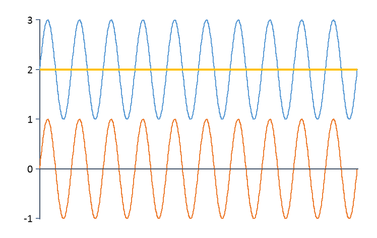
Constant |
Subtracts the mean value of the data set.
|
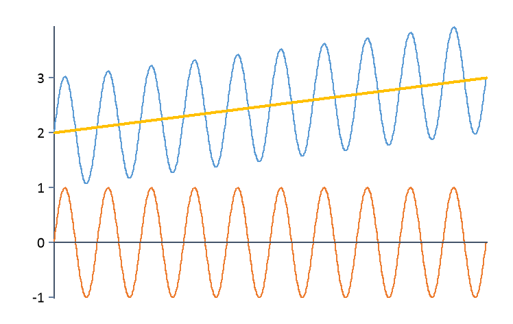
Linear |
Subtracts the best straight line, i.e., the straight line for which the sum of the squares of the deviations to the data set is minimal.
|
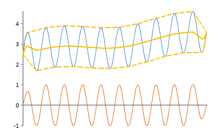
Adaptive |
Subtracts the mean value of the upper and lower envelope.
|
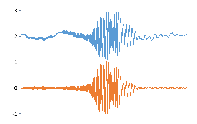
Moving average |
Subtracts the moving average. The interval width required to form the moving average can be entered. The setting can be used if the present trend is neither a constant nor linear, but time dependent. The moving average filter is a high-pass filter.
|
DC Offset Filter |
High-pass filter for removing the DC offset (IIR Butterworth high-pass). The cut-off frequency and the order (i.e. steepness) of the high-pass filter can be configured. The filter can be used if the present trend is neither a constant nor linear, but time dependent.
|
When determining the constant or linear trend, the mean value of the signal is first calculated and then the first and last level crossing through this value is searched for. If two level crossings are found, the mean value or the best straight line is calculated only for the range between these two level crossings. This prevents errors that occur at the end of the data set due to the phase cut-off of periodic signals. If no level crossings were found, then all values are included in the calculation. Suitable setting options for removing a time-dependent trend are usually subtraction of the moving average and the DC Offset Filter.
FPScript Functions Used
* This analysis object is not available in FlexPro View.