Integral (FPScript)
Calculates the integral.
Syntax
Integral(Signal [ , Mode = INTEGRAL_TRAPEZOIDAL ])
or
Integral(Amplitude, Time [ , Mode = INTEGRAL_TRAPEZOIDAL ])
The syntax of the Integral function consists of the following parts:
Part |
Description |
||||||||
|---|---|---|---|---|---|---|---|---|---|
Signal |
The signal whose integral is calculated. If the argument is a data series or a data matrix, then 1 is used as the increment dX for the integration. Permitted data structures are data series, data matrix, signal, signal series und signal series with two-dimensional X-component. All numeric data types are permitted. If the argument is a list, then the function is executed for each element of the list and the result is also a list. |
||||||||
Amplitude |
The Y component of the signal to be integrated. If you specify a signal, then its Y component is used. Permitted data structures are data series, data matrix, signal, signal series und signal series with two-dimensional X-component. All numeric data types are permitted. If the argument is a list, then the first element in the list is taken. If this is also a list, then the process is repeated. |
||||||||
Time |
The X component of the signal to be integrated. If you specify a signal, then its Y component is used. Permitted data structures are data series, data matrix, signal, signal series und signal series with two-dimensional X-component. All numeric data types are permitted. For complex data types the absolute value is formed. If the argument is a list, then the first element in the list is taken. If this is also a list, then the process is repeated. |
||||||||
Mode |
For the discrete calculation of the integral, approximation formulas with different orders of accuracy are used. The argument Mode can have the following values:
If the argument is a list, then the first element in the list is taken. If this is also a list, then the process is repeated. If this argument is omitted, it will be set to the default value INTEGRAL_TRAPEZOIDAL. |
Remarks
The result always has the data type 64-bit floating point.
The unit of the result is the same as the product of the units of the Signal Y and X components. The values are converted into 64-bit floating point values before the calculation is performed. For data matrices and signal series, the calculation takes place column by column. The X and Z components, if present, are copied into the result without modification. The result can be considered as a primitive function of the signal.
The integral is calculated in INTEGRAL_TRAPEZOIDAL mode with the help of the trapezoidal formula (at least two data points are required):
![]()
The trapezoidal rule can also be applied to non-equidistant sampled data sets.
The integral is calculated in INTEGRAL_SIMPSON mode with the help of the Simpson’s rule. The Simpson’s rule requires equidistantly sampled data sets (at least three data sets are required):
![]()
The integral is calculated in INTEGRAL_CUBIC mode with the help of a cubic integration formula. This integration rule is the centralized form of Adam’s integration rule (Adams interpolation formula or Ngo integrator, see [4].). The rule also requires equidistantly sampled data sets (at least four data sets are required):
![]()
In all modes the integral is defined at the left boundary I[0] as 0. In the case of the Simpson’s rule and the cubic integration rule, there are not enough sampling points for the approximation formula at the boundaries I[1] (and for the cubic rule also for the right-hand boundary I[N]). At these points calculation rules are used which have the same order of accuracy (similar to [2, page 98]).
Note In general the following applies: The higher the order of accuracy when choosing the integration rule, the greater the accuracy in determining the integral for smooth (non-noisy) data sets. However, if the data sets are noisy, the numerical error will be worse in determining the integral if a higher-order integration rule is used. The integration mode should therefore be selected based on the noise/smoothness of the underlying data set.
On the other hand, if one is interested in the frequency spectrum, it helps to consider the integration rules as digital filters (see also [1] or [3, section 7.2]). The integration rules have the following amplitude response. The ideal integrator is also displayed (filter profile of continuous integration):
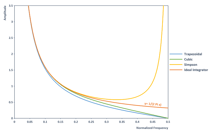
Observation: The trapezoidal rule and the cubic integration rule have natural low-pass characteristics and suppress high-frequency noise by underestimating the ideal integrator. The cubic integration rule has a more accurate amplitude response approximation of the ideal integrator than the trapezoidal rule throughout the entire frequency domain. The Simpson’s rule provides the most accurate amplitude response approximation of the ideal integrator in the frequency domain up to 0.25, but diverges in the area of the Nyquist limit 0.5. High-frequency noise is thus amplified using the Simpson’s rule. It should be noted that all approximation rules have a constant phase response of -90 degrees and thus match the phase of the ideal integrator.
Available in
FlexPro View, Basic, Professional, Developer Suite
Examples
Integral({1,2,3,2,1}, {0,1,2,3,4})
Uses the trapezoidal rule to calculate the integral {0, 1.5, 4, 6.5, 8} of the data series specified as the argument.
Integral(Signal)[-1]
Calculates the area under the curve of a signal. To do this, the last value must be taken from the result.
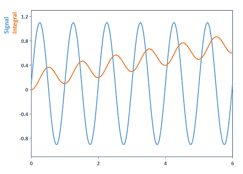
Integral(Detrend(Signal))
Integrates a periodic signal and removes the mean value in advance. In this case, the Detrend function was used to remove the DC component or a linear or adaptive trend from the signal before integration. Reason: When you integrate periodic signals that have a non-zero mean, then the integrated curve drifts away through accumulation of the mean value in the signal. The following illustration clarifies the situation:
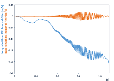
Integral(DCRemovalFilter(Signal))
Integrates a signal and removes the drift or offset (DC component) in advance. To remove the drift or offset, the DCRemovalFilter function was used instead of the Detrend function. Reason: The reason for this signal drifting after integration is not only the accumulation of the offset during integration, but also the integrator’s inversely proportional amplitude response to the frequency. This amplifies the noise at frequencies close to the offset (DC component) and integration raises it to arbitrarily high values. The integrated curve then drifts away. To prevent this drifting, it is not enough just to subtract the mean, but frequencies close to the DC component also need to be cut off using a high-pass filter. The following illustration clarifies the situation (here of one of the acceleration signals from the FlexPro example files under C:\Users\Public\Documents\Weisang\FlexPro were integrated):
Dim filterCoef = List("b", {1/3, 4/3, 1/3}, "a", {1, 0, -1})
AmplitudeResponse(filterCoef)
Calculates the amplitude response of the Simpson filter using the AmplitudeResponse function.
Dim x = Series(0, 6, 0.5)
Integral(Signal(2.2 + 6.2*x + 12.6*x^2 - 2*x^3, x), INTEGRAL_CUBIC)
Calculates the integral of a third degree polynomial at the x sampling points. The result agrees with the exact integral Signal(2.2*x + 3.1*x^2 + 4.2*x^3 - 0.5*x^4, x) .
Dim x = (30, 1, 0.1)
Dim f = Signal(50 * 1/x, x)
Dim integralExact = Signal(50 * log(x), x)
Absolute(Integral(f, INTEGRAL_TRAPEZOIDAL)[-1] - integralExact[-1])
Determines the error for the INTEGRAL_TRAPEZOIDAL mode when calculating the numerical integral of the smooth function f = 50 * 1 / x. The error is proportional to 0.01. On the other hand, if INTEGRAL_SIMPSON is selected, this yields an error proportional to 0.001. Selecting INTEGRAL_CUBIC returns the highest accuracy with an error proportional to 0.0001.
See Also
SavitzkyGolayDerivative Function
Signal Analysis - Analysis Object
References
[1] Tilman Butz: Fourier Transformation for Pedestrians. Springer Berlin Heidelberg New York,http://www.springer.com/de/book/9783319169842,2015.ISBN 3-540-23165-X.
[2] C. Woodford, C. Phillips: Numerical Methods with Worked Examples. Chapman and Hall, 2-6 Boundary Row, London SE1 8HN, UK,1997.ISBN 0-412-72150-3.
[3] Richard G. Lyons: Understanding Digital Signal Processing (3rd Edition). Prentice Hall,2011.ISBN 0-13-702741-9.
[4] N. Q. Ngo: A new approach for the design of wideband digital integrator and differentiator. In: IEEE Trans. Circuits Syst. II, Exp. Briefs, Vol. 53, No. 9, Pages 936-940. Prentice Hall,2006.