Spline Interpolation Analysis Object *
You can use this analysis object to perform a spline interpolation for your data, i.e., to calculate a smooth curve that connects the points in your data set. Spline interpolation is directly integrated into the line plot of FlexPro so that you only use this analysis object when you want to process smoothed data further mathematically.
With spline interpolation, all neighboring points of the curve are connected by polynomials of the third degree, i.e. functions of the form:
![]()
Two polynomials meet at each point of the curve. The first and last point in the curve form the exception. The coefficients ai, bi, ci and di of the polynomials are selected such that the neighboring polynomials agree in locus, gradient and curvature at the places where they meet. For the first and last point where no polynomials meet, you can change the appearance of the spline curve using what are called boundary conditions, i.e. you specify either gradient or curvature of the spline curve at the left and right edges. Depending on the type of boundary conditions, you obtain a different appearance of the spline curve, as shown in the following illustration:
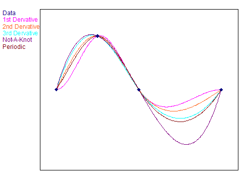
This highlights:
•Natural splines. You obtain these when you select Curvatures as specified as the boundary condition and enter the value zero for the values for the curvatures at both edges. The appearance corresponds to the curve that you would obtain if you were to connect the points of the curve using a rubber ruler.
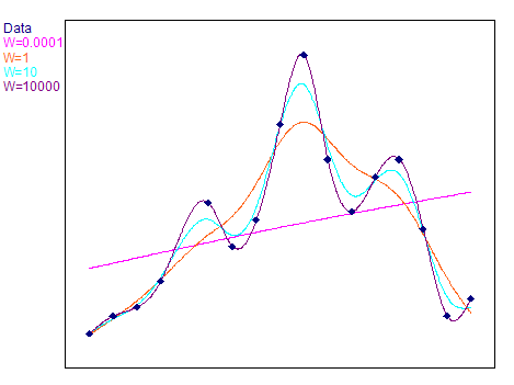
•Compensating splines. The curve calculated in this way does not necessarily pass through the specified sampling points. The curve ripple can be controlled using a weighting factor. If the weighting factor is close to zero, the spline curve results in the best straight line with respect to the square error. For a very large weighting factor, you obtain a natural spline curve, which corresponds with the boundary conditions specified above. In this case, the course of the spline curve follows the points of the curve.
•Periodic splines originate from the demand that the spline curve must agree in gradient and curvature at the left and right edges. You can then tag the resulting spline curves onto each other several times in succession, without kinks developing at the joints. To calculate a periodic spline interpolation, the Y values from the first and last points must be the same. If this is not the case, FlexPro uses one of two methods to force the periodicity. If you select Periodic, periodicity by replacement, the last Y value in the data set is ignored and a copy of the first Y value is used instead. However, if you select Periodic, periodicity by appending, a copy of the first Y value is appended to the data set if the last Y value in the data set is not identical to the first Y value. The X value of the original last point plus the difference between the last and next to last X value is used as the X value for this extra point.
•Splines with a "Not-A-Knot" boundary condition. These use two identical polynomials, one on the left and one right edge, which corresponds to the condition that the third derivative of the Spline functions in the second and second to the last data points are continuous. This means that these points are not true nodal points on the spline curve.
The pre-condition for the spline interpolation is that the X values of the points are strictly increasing. If this is not the case, (e.g., with a locus curve), then you should use parametric spline interpolation. The X values, however, do not have to be equidistant. After the coefficients of the spline curve are calculated, FlexPro can evaluate the spline function calculated at any points to obtain new sampling points.
The following illustration shows compensating splines with different weighting factors:
The result of the spline interpolation is first a mathematical model of the data set to be interpolated. Theevaluation mode specifies at which points the calculated spline curve is to be evaluated to obtain the result data set. The following evaluation modes are possible:
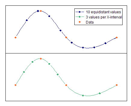
•N-values equidistant: In this case, the spline curve is evaluated at N equidistant sampling points, irrespective of how the X values were previously distributed.
•N-values per X interval: In this case, each previous X Interval is divided into N equally-sized intervals, at whose limits the spline function is evaluated.
The following illustration shows how the two evaluation modes operate:
FPScript Functions Used
See Also
Parametric Spline Interpolation Analysis Object
Linear Interpolation Analysis Object
* This analysis object is not available in FlexPro View.