Derivative (FPScript)
Calculates the first derivative.
Syntax
Derivative(Signal [ , Mode = DERIVATIVE_CENTRAL_3_POINTS ])
or
Derivative(Amplitude, Time [ , Mode = DERIVATIVE_CENTRAL_3_POINTS ])
The syntax of the Derivative function consists of the following parts:
Part |
Description |
||||||
|---|---|---|---|---|---|---|---|
Signal |
The signal whose first derivative is calculated. If the argument is a data series or data matrix, 1 is used as the increment dX for the derivative. Permitted data structures are data series, data matrix, signal, signal series und signal series with two-dimensional X-component. All numeric data types are permitted. If the argument is a list, then the function is executed for each element of the list and the result is also a list. |
||||||
Amplitude |
Returns the Y component of the signal to be processed. If you specify a signal, its Y component is used. Permitted data structures are data series, data matrix, signal, signal series und signal series with two-dimensional X-component. All numeric data types are permitted. If the argument is a list, then the first element in the list is taken. If this is also a list, then the process is repeated. |
||||||
Time |
Returns the X component of the signal to be processed. If you specify a signal, its Y component is used. Permitted data structures are data series, data matrix, signal, signal series und signal series with two-dimensional X-component. All numeric data types are permitted. For complex data types the absolute value is formed. If the argument is a list, then the first element in the list is taken. If this is also a list, then the process is repeated. |
||||||
Mode |
For the discrete approximation of the derivative, finite differences in the form of central difference quotients are used. The order of the finite differences used determines the accuracy for the numerical calculation of the derivative. The argument Mode can have the following values:
If the argument is a list, then the first element in the list is taken. If this is also a list, then the process is repeated. If this argument is omitted, it will be set to the default value DERIVATIVE_CENTRAL_3_POINTS. |
Remarks
The result always has the data type 64-bit floating point.
The unit of the result is equal to the quotient of the units of Amplitude and Time or of the Y and X components of Signal. For data matrices and signal series, the calculation takes place column by column. The values are converted to 64-bit floating points before the calculation is made. If present, the X or Z components are copied to the result unchanged. The numerical derivative is calculated in DERIVATIVE_CENTRAL_3_POINTS mode for equidistantly sampled data sets (increment dX) with the help of the following central difference quotients (at least three data points required):
![]()
This corresponds to averaging the left-sided and right-sided (one-sided) difference quotients, i.e.:
![]()
In DERIVATIVE_CENTRAL_5_POINTS mode, the numerical derivative for equidistantly sampled data sets (increment dX) is calculated with the help of the following central difference quotients (at least five data points required):
![]()
For both variants there are not enough sampling points at the boundaries to calculate the central differences. There, the numerical derivative is therefore calculated using non-central finite difference quotients of the same order. The algorithms at the boundaries are specified in [1].
The specified algorithms of the numerical derivative can also be generalized for non-equidistantly sampled data sets; see [1]. These algorithms are also implemented in FlexPro and are used automatically as soon as that the underlying data set has non-equidistant sampling.
Note In general the following applies: The higher the order when selecting the finite differences, the greater the accuracy in determining the derivative for smooth (non-noisy) data sets. However, if the data sets are noisy, the numerical error will be worse in determining the derivative if a higher order finite differences rule is used. The derivation mode should therefore be selected based on the noise/smoothness of the underlying data set. For example, the DERIVATIVE_CENTRAL_5_POINTS mode is required for crash analyses; see guidelines J1727 from [2] and ECE-R94 from [3].
On the other hand, if one is interested in the frequency spectrum, it helps to consider the derivative rules as digital filters (see [4]). The derivative rules have the following amplitude response. The ideal differentiator is also displayed (filter profile of continuous differentiation) as well as the forward and backward differentiation using the Diff function.
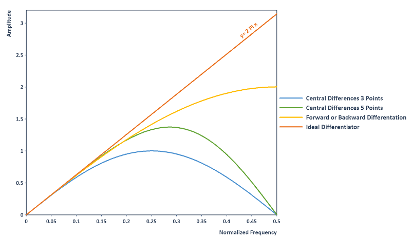
Observation: The central 3-point rule and central 5-point rule suppress high-frequency noise in the Nyquist limit 0.5. The central 5-point rule has a more precise amplitude response approximation of the ideal differentiator over the entire frequency domain than the central 3-point rule. The one-sided forward and backward difference quotients may also have a more precise amplitude response approximation of the ideal differentiator, but amplify the high-frequency noise as a result. It should be noted that the central difference rules have a constant phase response of 90 degrees and thus precisely match the phase response of the ideal differentiator. On the other hand, the forward and backward difference quotients have a linear phase shift.
Available in
FlexPro View, Basic, Professional, Developer Suite
Examples
Derivative(Signal)
Calculates the discrete derivative of an arbitrary signal with the help of the central 3-point rule.
Derivative({1.0, 3.0, 5.0, 5.0, 4.0, 3.0})
Calculates the derivative {2, 2, 1, -0.5, -1, -1} of the data series specified as the argument, where 1.0 is used as the increment dX. The result has the same data set length as the input data set.
Diff({1.0, 3.0, 5.0, 5.0, 4.0, 3.0}, DIFF_QUOTIENT_FORWARD)
Calculates the difference quotients of neighboring values using the Diff function and produces {2, 2, 0, -1, -1} as the result. The Diff function uses (first order) non-central finite differences. Hence the data set length of the result is reduced by one compared to the input data set.
Dim x = Series(-6, 6, 0.5)
Derivative(Signal(2.2 + 6.1*x + 3.6*x^2 + 12*x^3 - x^4, x), DERIVATIVE_CENTRAL_5_POINTS)
Calculates the derivative of a fourth degree polynomial at the sampling points x. The result coincides with the exact derivative Signal(6.1 + 7.2*x + 36*x^2 - 4*x^3, x).
Dim x = Series(-3, 3, 0.1)
Dim f = Signal(Sin(x^2), x)
Dim derivExact = Signal(2*x*Cos(x^2), x)[[ 1.0 ]]
Absolute(Derivative(f, DERIVATIVE_CENTRAL_3_POINTS)[[ 1.0 ]] - derivExact)
Determines the error for the DERIVATIVE_CENTRAL_3_POINTS mode when calculating the numerical derivative of the smooth function f = Sin(x2) at the point 1.0. The error is proportional to 0.01. On the other hand, if DERIVATIVE_CENTRAL_5_POINTS is selected, this yields greater accuracy with an error proportional to 0.0001. However, if the Diff function is used, the derivative is calculated with an error proportional to 0.1 (lowest accuracy). For approximation of the derivative, the Derivative function should therefore be used instead of the Diff function.
See Also
SavitzkyGolayDerivative Function
Signal Analysis - Analysis Object
References
[1] Bengt Fornberg: Generation of Finite Difference Formulas on Arbitrarily Spaced Grids. In: Mathematics of Computation, Vol. 51, No. 184, Pages 699-706. https://doi.org/10.1090/S0025-5718-1988-0935077-0,1988.
[2] Safety Test Instrumentation Stds Comm: Calculation Guidelines for Impact Testing (J1727). In: SAE International. http://standards.sae.org/j1727_201502/,2015.
[3] UN Vehicle Regulations: Regulation No. 94 - Frontal collision protection (ECE-R94). In: Concerning the Adoption of Uniform Technical Prescriptions for Wheeled Vehicles, Equipment and Parts which can be Fitted and/or be Used on Wheeled Vehicles and the Conditions for Reciprocal Recognition of Approvals Granted on the Basis of these Prescriptions. http://www.unece.org/trans/main/wp29/wp29regs81-100.html,2013.
[4] Tilman Butz: Fourier Transformation for Pedestrians. Springer Berlin Heidelberg New York,http://www.springer.com/de/book/9783319169842,2015.ISBN 3-540-23165-X.