Calculates the autocorrelation function of a signal. Describes the similarity of a signal to itself.

Syntax

ACF(Signal [ , Mode = CORRELATIONPRODUCT_NONCIRCULAR ])

The syntax of the ACF function consists of the following parts:

Remarks

The data type of the result is always 64-bit floating point.

The structure of the result corresponds to that of the argument Signal.

The unit of the result is the same as the square of the unit of Signal. The autocorrelation for a data series s is defined as:

with the correlation product:

and N, the number of values in s.

The values of the normalized autocorrelation are between -1 und +1. The normalized correlation calculates the quotient between autocorrelation and the product of the RMS values of the input data sets.

The calculation occurs in the frequency domain in all cases according to the following formula:

IRFFTn(*FFTn(Signal) * FFTn(Signal))

For two-dimensional arguments, the calculation is carried out column by column, and the result is also two-dimensional. If one of the arguments has an X component, this also applies to the result.

For a circular autocorrelation, the calculation takes place under the assumption that one or more complete periods of the signal are stored in the data set. If the result has an X component, then this component contains the τ time lag of the autocorrelation function. The value τ = 0 is always located exactly at the beginning of the X data series. Therefore, no negative τ values are calculated. Due to the periodicity of autocorrelation, the values in the second half of the result can, however, also be regarded as negative τ values in this case.

The non-circular autocorrelation is based on the assumption that the signal outside of the section covered by the Signal data set amounts to zero. A sufficient number of zeros is therefore appended to the data set before transformation into the frequency domain. The autocorrelation function is calculated for all τ values for which this can have a value not equal to zero, i.e., for which there is still an overlap of the signal with its shifted copy. If the result has an X component, then this component contains the τ time lag of the autocorrelation function. The value τ = 0 is always exactly in the center of the X data series.

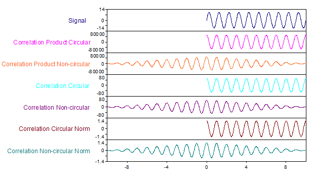
The following illustration shows different variations for a sinusoidal signal with a frequency of 1, amplitude of 10 and an X range from 0 to 10:

Available in

FlexPro Basic, Professional, Developer Suite

Examples

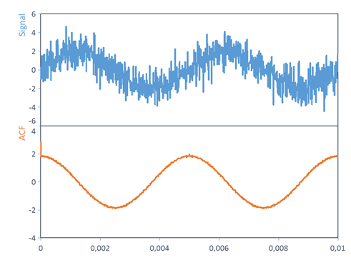
ACF(Signal(2. * Sin(2. * PI * 200. * (1000, 0., 1.e-005)) + Noise((1000, 0., 1.e-005), NOISE_NORMAL), (1000, 0., 1.e-005)), CORRELATION_CIRCULAR)

There is a sinusoidal signal with a frequency f = 200 Hz, amplitude = 2 V, phase = 0° and offset = 0 V above two periods. The signal is superimposed with a Gaussian noise (mean value μ = 0 V, standard deviation σ = 1 V).

Using the autocorrelation function ACF , the amplitude and frequency of the disturbed periodic signal is now recovered.

See Also

CCF Function

Correlation Function

Correlation Analysis Object

References

[1] "Oppenheim, A. V. and Schafer, R. W.": "Discrete-Time Signal Processing, 2nd Edition", page 743 - 48. "Prentice Hall, New Jersey",1999.ISBN 0-13-754920-2.

[2] "H.D. Lüke": "Signalübertragung (Signal Transmission)", page 79 - 81. "Springer-Verlag Berlin, Heidelberg, New York",1985.ISBN 3-540-15526-0.